| Learning Objective | Essential Knowledge |
|---|---|
1.1.A |
|
1.1.B |
|
Tips
AP Precalculus covers polynomial and rational functions, exponential and logarithmic functions, trigonometric and polar functions, and an introduction to vectors, matrices and parametric functions. It is the bridge into calculus, and the exam is unusually strict about how you describe a function.
Describing change is the whole course. Expect to say where a function increases or decreases, how fast, and whether that rate is itself increasing — in a full sentence, with the correct vocabulary.
Learn the parent functions and their transformations cold. Everything else in the course is built from them, and recognising a shifted or stretched parent instantly is what makes the harder questions short.
Notes follow the four CED units — polynomial and rational, exponential and logarithmic, trigonometric and polar, and functions involving parameters — each with worked examples. Sample exam questions are in the library. Precalculus asks you to describe how a function behaves in sentences, which the examples model.
-
1
Polynomial and Rational Functions
Watch lesson1.1
Change in Tandem
Syllabus
Source: College Board AP Course and Exam Description
A function 函数 is a rule that maps each input to exactly one output. The set of allowed inputs is the domain 定义域; the set of outputs is the range 值域. The input variable is the independent variable 自变量 and the output variable is the dependent variable 因变量. A function rule can be shown graphically, numerically, analytically (a formula), or verbally.
As the input changes, the output changes "in tandem" – together. Over an interval, a function is:
- increasing 递增 if, whenever $a
- decreasing 递减 if, whenever $a
A graph of a function shows all its input–output pairs, so you can read this behavior straight off the picture.
ExploreWatch two quantities change together
y = ax² + bx + c
Precalculus studies how an output changes in tandem with its input. Read the curve left to right: where it is steep, $y$ changes a lot for a small change in $x$; where it is flat, $y$ barely moves.
Vocabulary TrainEnglish function/ˈfʌŋkʃn/ domain/dəˈmeɪn/ range/reɪndʒ/ independent variable/ˌɪndɪˈpendənt ˈveərɪəbl/ dependent variable/dɪˈpendənt ˈveərɪəbl/ increasing/ɪnˈkriːsɪŋ/ decreasing/ˈdiːkriːsɪŋ/ 1.2
Rates of Change
Syllabus
Learning Objective Essential Knowledge 1.2.A
Compare the rates of change at two points using average rates of change near the points.- 1.2.A.1 The average rate of change of a function over an interval of the function's domain is the constant rate of change that yields the same change in the output values as the function yielded on that interval of the function's domain. It is the ratio of the change in the output values to the change in input values over that interval.
- 1.2.A.2 The rate of change of a function at a point quantifies the rate at which output values would change were the input values to change at that point. The rate of change at a point can be approximated by the average rates of change of the function over small intervals containing the point, if such values exist.
- 1.2.A.3 The rates of change at two points can be compared using average rate of change approximations over sufficiently small intervals containing each point, if such values exist.
1.2.B
Describe how two quantities vary together at different points and over different intervals of a function.- 1.2.B.1 Rates of change quantify how two quantities vary together.
- 1.2.B.2 A positive rate of change indicates that as one quantity increases or decreases, the other quantity does the same.
- 1.2.B.3 A negative rate of change indicates that as one quantity increases, the other decreases.
Source: College Board AP Course and Exam Description
The average rate of change 平均变化率 of a function over an interval is the change in output divided by the change in input – the single constant rate that would give the same total change. Over $[a,b]$:
$$\text{avg rate} = \frac{f(b)-f(a)}{b-a}.$$The rate of change at a point measures how fast the output changes right at that input. You approximate it with average rates over small intervals around the point. Comparing two points, the one with the larger average rate (over small enough intervals) is changing faster. A positive rate means both quantities move the same way; a negative rate means they move in opposite ways.
Worked example. For $f(x)=x^2$, the average rate of change over $[1,4]$ is $\dfrac{f(4)-f(1)}{4-1}=\dfrac{16-1}{3}=5$. Over $[1,2]$ it is $\dfrac{4-1}{1}=3$ – the rate itself changes, which is exactly why $f$ is not linear.
Vocabulary TrainEnglish average rate of change/ˈævrɪdʒ reɪt ɒv tʃeɪndʒ/ 1.3
Rates of Change in Linear and Quadratic Functions
Syllabus
Learning Objective Essential Knowledge 1.3.A
Determine the average rates of change for sequences and functions, including linear, quadratic, and other function types.- 1.3.A.1 For a linear function, the average rate of change over any length input-value interval is constant.
- 1.3.A.2 For a quadratic function, the average rates of change over consecutive equal-length input-value intervals can be given by a linear function.
- 1.3.A.3 The average rate of change over the closed interval $[a, b]$ is the slope of the secant line from the point $(a, f(a))$ to $(b, f(b))$.
1.3.B
Determine the change in the average rates of change for linear, quadratic, and other function types.- 1.3.B.1 For a linear function, since the average rates of change over consecutive equal-length input-value intervals can be given by a constant function, these average rates of change for a linear function are changing at a rate of zero.
- 1.3.B.2 For a quadratic function, since the average rates of change over consecutive equal-length input-value intervals can be given by a linear function, these average rates of change for a quadratic function are changing at a constant rate.
- 1.3.B.3 When the average rate of change over equal-length input-value intervals is increasing for all small-length intervals, the graph of the function is concave up. When the average rate of change over equal-length input-value intervals is decreasing for all small-length intervals, the graph of the function is concave down.
Source: College Board AP Course and Exam Description
The average rate of change over $[a,b]$ is the slope of the secant line 割线 from $(a,f(a))$ to $(b,f(b))$.
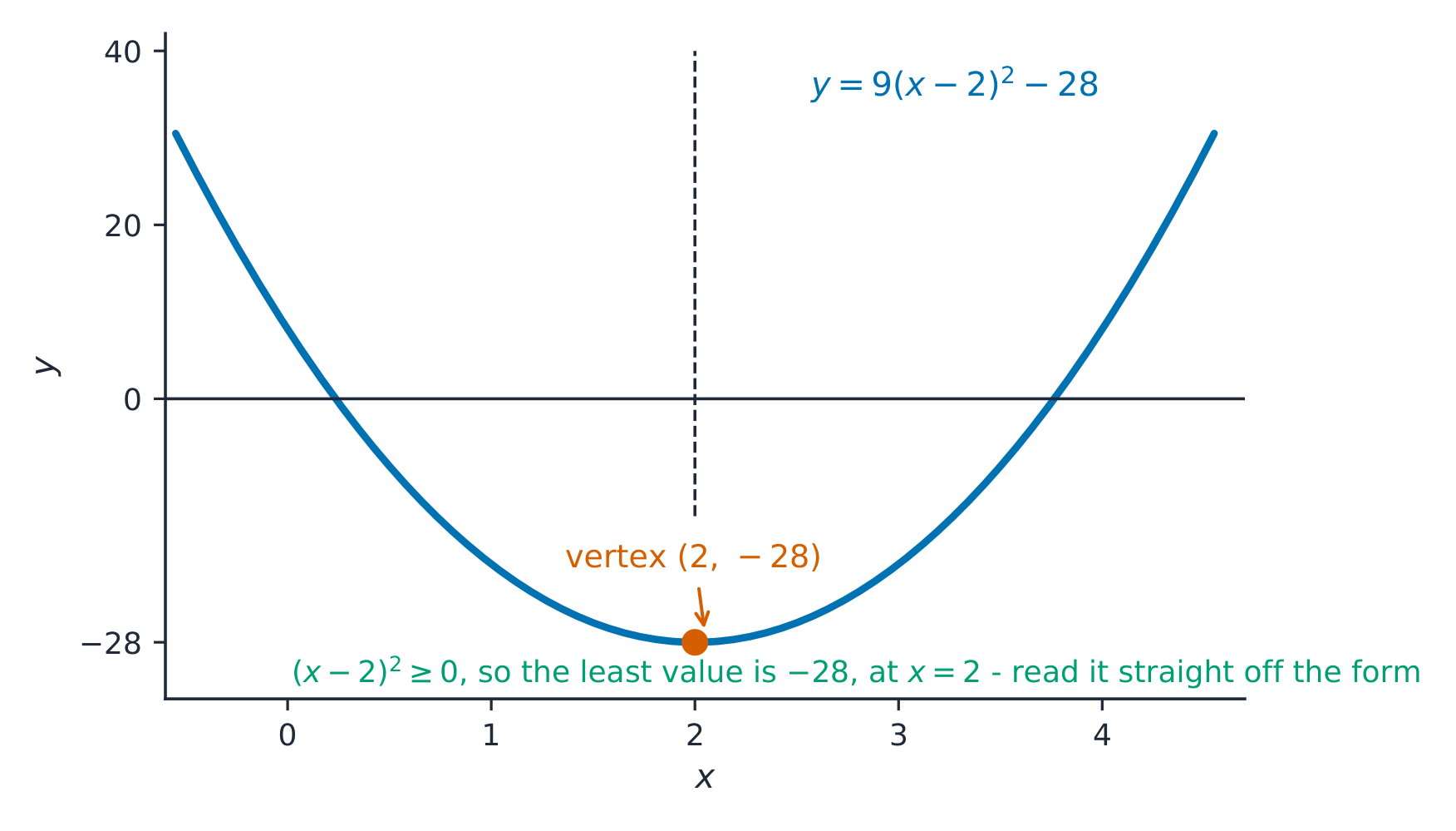
Completing the square gives the vertex of a parabola - For a linear 线性 function, the average rate of change over any interval is constant – so the rate at which the rate changes is zero.
- For a quadratic 二次 function, the average rates of change over equal-length intervals themselves form a linear pattern – so those rates change at a constant rate.
This "rate of the rate" idea distinguishes function types: a constant second difference signals a quadratic.

A hanging bridge cable takes the shape of a parabola-like curve — a quadratic you can see in steel ExploreExplore a quadratic's changing rate
y = ax² + bx + c
Move the sliders and watch the parabola 抛物线 tilt. Its average rate of change is not constant — the slope is positive on one side of the vertex 顶点 and negative on the other. Notice how $a$ opens it up or down.
Vocabulary TrainEnglish secant line/ˈsiːkənt laɪn/ linear/ˈlɪnɪə/ quadratic/kwɒˈdrætɪk/ 1.4
Polynomial Functions and Rates of Change

Syllabus
Learning Objective Essential Knowledge 1.4.A
Identify key characteristics of polynomial functions related to rates of change.- 1.4.A.1 A nonconstant polynomial function of $x$ is any function representation that is equivalent to the analytical form $p(x) = a_n x^n + a_{n-1} x^{n-1} + a_{n-2} x^{n-2} + \ldots + a_2 x^2 + a_1 x + a_0$, where $n$ is a positive integer, $a_i$ is a real number for each $i$ from $1$ to $n$, and $a_n$ is nonzero. The polynomial has degree $n$, the leading term is $a_n x^n$, and the leading coefficient is $a_n$. A constant is also a polynomial function of degree zero.
- 1.4.A.2 Where a polynomial function switches between increasing and decreasing, or at the included endpoint of a polynomial with a restricted domain, the polynomial function will have a local, or relative, maximum or minimum output value. Of all local maxima, the greatest is called the global, or absolute, maximum. Likewise, the least of all local minima is called the global, or absolute, minimum.
- 1.4.A.3 Between every two distinct real zeros of a nonconstant polynomial function, there must be at least one input value corresponding to a local maximum or local minimum.
- 1.4.A.4 Polynomial functions of an even degree will have either a global maximum or a global minimum.
- 1.4.A.5 Points of inflection of a polynomial function occur at input values where the rate of change of the function changes from increasing to decreasing or from decreasing to increasing. This occurs where the graph of a polynomial function changes from concave up to concave down or from concave down to concave up.
Source: College Board AP Course and Exam Description
A smooth bridge curve: polynomial and rational graphs model real shapes with asymptotes and turns A nonconstant polynomial 多项式 has the form
$$p(x)=a_n x^n + a_{n-1}x^{n-1}+\cdots+a_1 x + a_0,\quad a_n\neq 0.$$Its degree 次数 is $n$, its leading term 首项 is $a_n x^n$, and its leading coefficient 首项系数 is $a_n$. A constant is a polynomial of degree $0$.Key features:
- Where a polynomial switches between increasing and decreasing, it has a local (relative) extremum 局部极值. The greatest local maximum is the global (absolute) maximum 全局最大值 only when the polynomial has one — but most polynomials are unbounded (every odd-degree polynomial runs off to $\pm\infty$), so they have no global maximum or minimum at all.
- Between any two distinct real zeros there is at least one local maximum or minimum.
- An even-degree polynomial has either a global maximum or a global minimum.
- A point of inflection 拐点 is where the graph changes concavity – from concave up 上凹 to concave down 下凹 or the reverse – i.e. where the rate of change switches between increasing and decreasing.
- A function has symmetry when it is even 偶函数 – $f(-x)=f(x)$, graph symmetric across the $y$-axis (like $x^2$, $x^4$) – or odd 奇函数 – $f(-x)=-f(x)$, graph symmetric by rotation about the origin (like $x^3$, $x^5$). Test by substituting $-x$ and simplifying; later, $\cos\theta$ is even and $\sin\theta$ is odd.
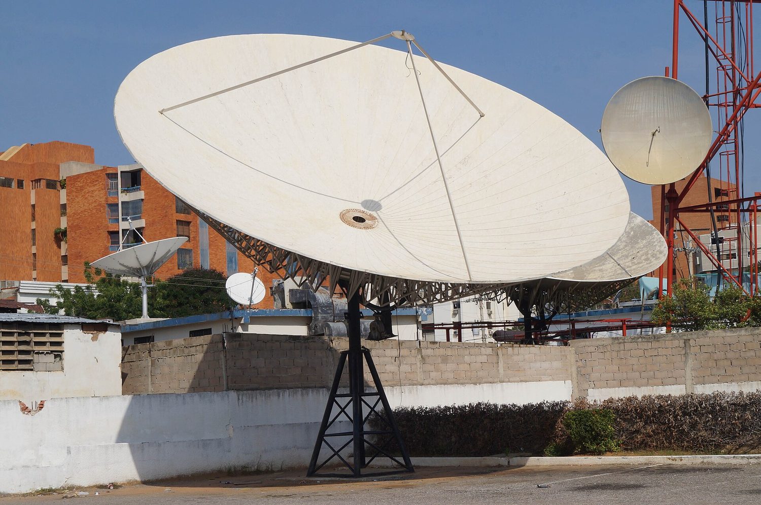
A satellite dish is a parabola of revolution: every parallel ray reflects to the same focus Vocabulary TrainEnglish polynomial/ˌpɒlɪˈnəʊmɪəl/ degree/dɪˈɡriː/ leading term/ˈliːdɪŋ tɜːm/ leading coefficient/ˈliːdɪŋ ˌkəʊɪˈfɪʃənt/ local (relative) extremum/ˈləʊkl ekˈstreməm/ global (absolute) maximum/ˈɡləʊbl ˈmæksɪməm/ point of inflection/pɔɪnt ɒv ɪnˈflekʃn/ concave up/kɒnˈkeɪv ʌp/ concave down/kɒnˈkeɪv daʊn/ even/ˈiːvən/ odd/ɒd/ 1.5
Polynomial Functions and Complex Zeros
Syllabus
Learning Objective Essential Knowledge 1.5.A
Identify key characteristics of a polynomial function related to its zeros when suitable factorizations are available or with technology.- 1.5.A.1 If $a$ is a complex number and $p(a) = 0$, then $a$ is called a zero of the polynomial function $p$, or a root of $p(x) = 0$. If $a$ is a real number, then $(x - a)$ is a linear factor of $p$ if and only if $a$ is a zero of $p$.
- 1.5.A.2 If a linear factor $(x - a)$ is repeated $n$ times, the corresponding zero of the polynomial function has a multiplicity $n$. A polynomial function of degree $n$ has exactly $n$ complex zeros when counting multiplicities.
- 1.5.A.3 If $a$ is a real zero of a polynomial function $p$, then the graph of $y = p(x)$ has an $x$-intercept at the point $(a, 0)$. Consequently, real zeros of a polynomial can be endpoints for intervals satisfying polynomial inequalities.
- 1.5.A.4 If $a + bi$ is a non-real zero of a polynomial function $p$, then its conjugate $a - bi$ is also a zero of $p$.
- 1.5.A.5 If the real zero, $a$, of a polynomial function has even multiplicity, then the signs of the output values are the same for input values near $x = a$. For these polynomial functions, the graph will be tangent to the $x$-axis at $x = a$.
- 1.5.A.6 The degree of a polynomial function can be found by examining the successive differences of the output values over equal-interval input values. The degree of the polynomial function is equal to the least value $n$ for which the successive $n$th differences are constant.
1.5.B
Determine if a polynomial function is even or odd.- 1.5.B.1 An even function is graphically symmetric over the line $x = 0$ and analytically has the property $f(-x) = f(x)$. If $n$ is even, then a polynomial of the form $p(x) = a_n x^n$, where $n \geq 1$ and $a_n \neq 0$, is an even function.
- 1.5.B.2 An odd function is graphically symmetric about the point $(0, 0)$ and analytically has the property $f(-x) = -f(x)$. If $n$ is odd, then a polynomial of the form $p(x) = a_n x^n$, where $n \geq 1$ and $a_n \neq 0$, is an odd function.
Source: College Board AP Course and Exam Description
A zero 零点 (or root 根) of $p$ is a number $a$ with $p(a)=0$. For a real $a$, $(x-a)$ is a factor of $p$ exactly when $a$ is a zero. If the factor $(x-a)$ is repeated $n$ times, that zero has multiplicity 重数 $n$. Counting multiplicities, a degree-$n$ polynomial has exactly $n$ complex 复数 zeros.
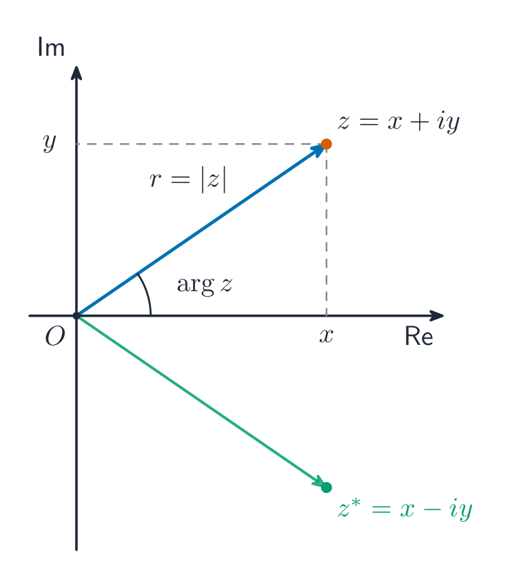
A complex number on an Argand diagram: modulus is the distance, argument the angle - A real zero $a$ gives an $x$-intercept at $(a,0)$; real zeros are the endpoints of the intervals where $p(x)\ge 0$ or $\le 0$.
- Non-real zeros come in conjugate 共轭 pairs: if $a+bi$ is a zero, so is $a-bi$.
- At a real zero of even multiplicity the graph is tangent to the $x$-axis (it touches but does not cross); at odd multiplicity it crosses.
- The degree equals the least $n$ for which the $n$th successive differences of equally-spaced outputs become constant.
Vocabulary TrainEnglish zero/ˈzɪərəʊ/ root/ruːt/ multiplicity/ˌmʌltɪˈplɪsɪti/ complex/ˈkɒmpleks/ conjugate/ˈkɒndʒuːɡeɪt/ 1.6
Polynomial Functions and End Behavior
Syllabus
Learning Objective Essential Knowledge 1.6.A
Describe end behaviors of polynomial functions.- 1.6.A.1 As input values of a nonconstant polynomial function increase without bound, the output values will either increase or decrease without bound. The corresponding mathematical notation is $\lim_{x \to \infty} p(x) = \infty$ or $\lim_{x \to \infty} p(x) = -\infty$.
- 1.6.A.2 As input values of a nonconstant polynomial function decrease without bound, the output values will either increase or decrease without bound. The corresponding mathematical notation is $\lim_{x \to -\infty} p(x) = \infty$ or $\lim_{x \to -\infty} p(x) = -\infty$.
- 1.6.A.3 The degree and sign of the leading term of a polynomial determines the end behavior of the polynomial function, because as the input values increase or decrease without bound, the values of the leading term dominate the values of all lower-degree terms.
Source: College Board AP Course and Exam Description
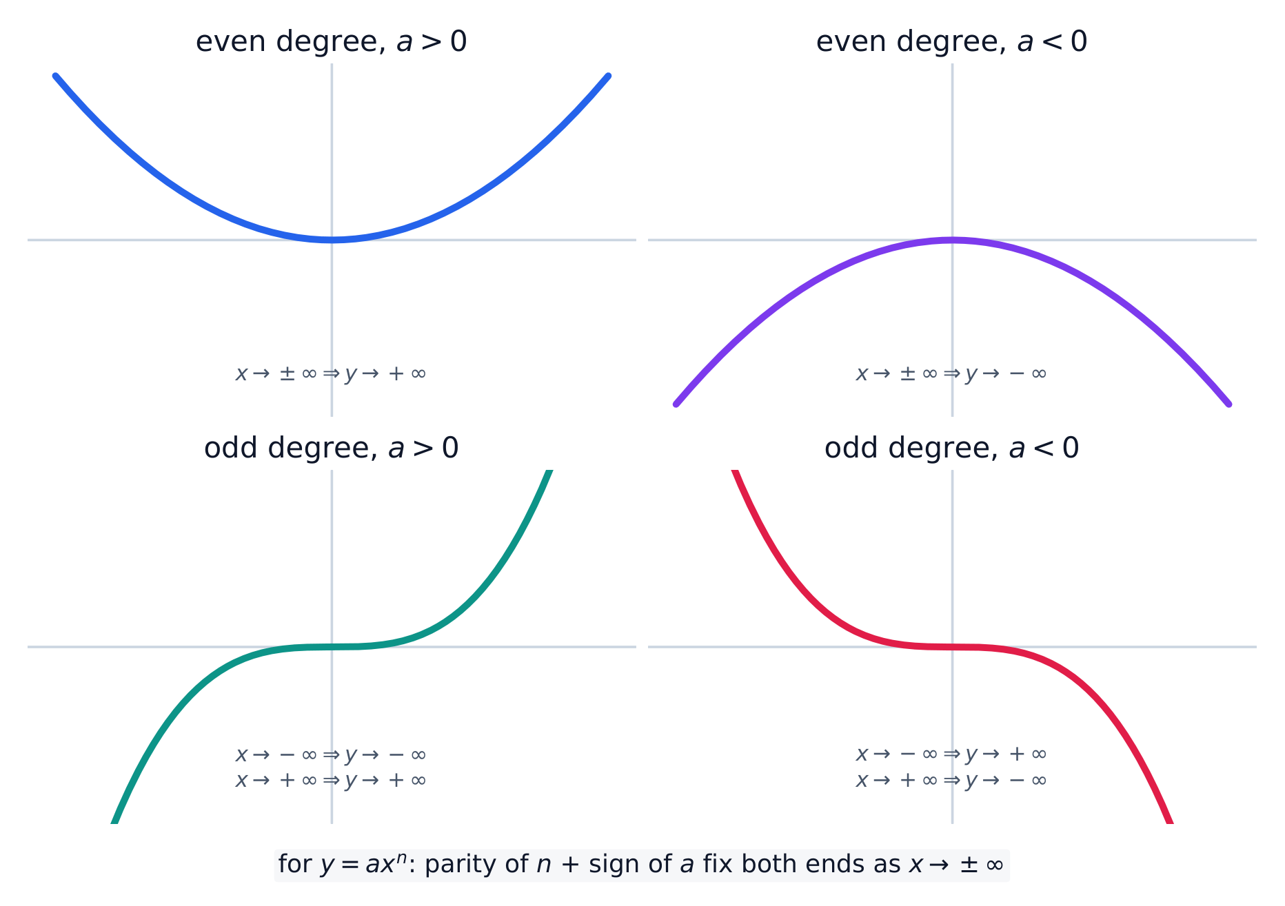
End behavior 末端行为 describes where a function heads as the input grows without bound. For a nonconstant polynomial, as $x\to\pm\infty$ the output goes to $+\infty$ or $-\infty$, written e.g. $\lim_{x\to\infty}p(x)=\infty$. Which way depends entirely on the leading term $a_n x^n$, because for large $|x|$ it dominates all lower-degree terms: the sign of $a_n$ and whether $n$ is even or odd fix both ends.
Every polynomial's ends are decided by its degree's parity and the sign of its leading coefficient ExploreSee how the leading term sets the end behavior
y = ax³ + bx² + cx + d
The leading term decides the ends. For a cubic with $a>0$ the graph falls on the left and rises on the right; make $a<0$ and the two ends swap. As $x\to\pm\infty$ the highest-power term dominates every other term.
Vocabulary TrainEnglish End behavior/end bɪˈheɪvjə/ 1.7
Rational Functions and End Behavior
Syllabus
Learning Objective Essential Knowledge 1.7.A
Describe end behaviors of rational functions.- 1.7.A.1 A rational function is analytically represented as a quotient of two polynomial functions and gives a measure of the relative size of the polynomial function in the numerator compared to the polynomial function in the denominator for each value in the rational function's domain.
- 1.7.A.2 The end behavior of a rational function will be affected most by the polynomial with the greater degree, as its values will dominate the values of the rational function for input values of large magnitude. For input values of large magnitude, a polynomial is dominated by its leading term. Therefore, the end behavior of a rational function can be understood by examining the corresponding quotient of the leading terms.
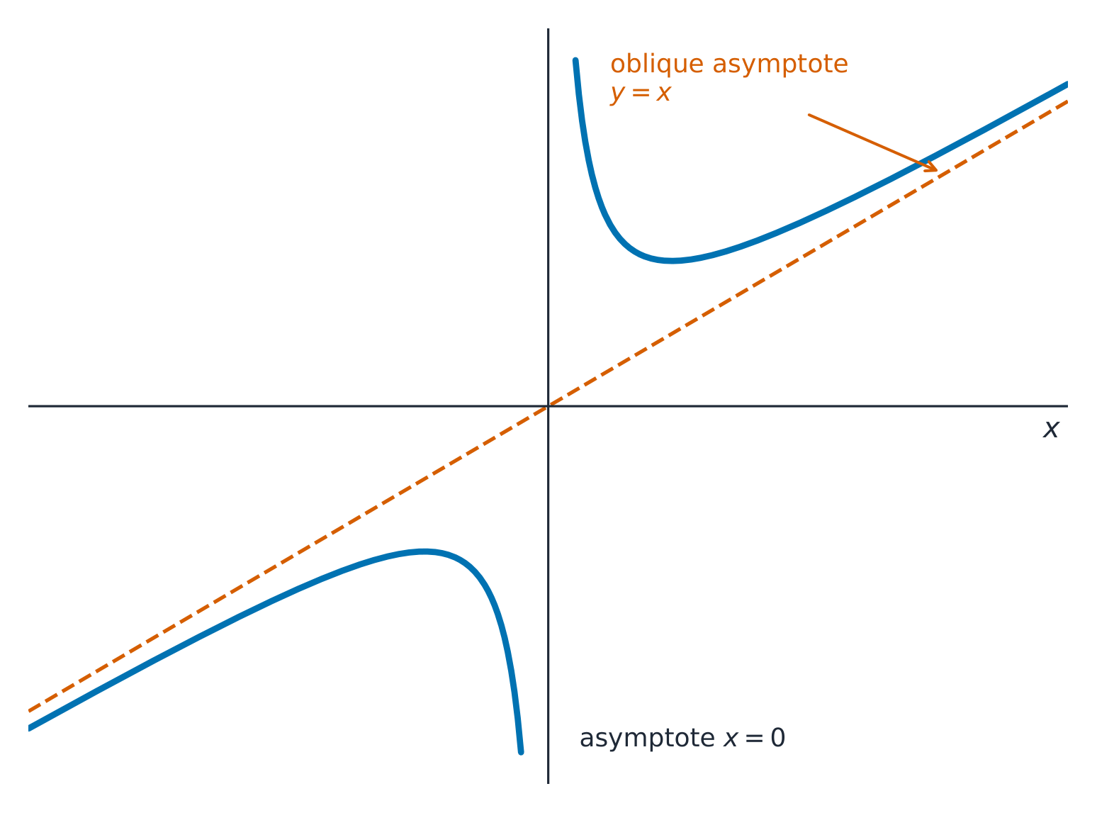
- 1.7.A.3 If the polynomial in the numerator dominates the polynomial in the denominator for input values of large magnitude, then the quotient of the leading terms is a nonconstant polynomial, and the original rational function has the end behavior of that polynomial. If that polynomial is linear, then the graph of the rational function has a slant asymptote parallel to the graph of the line.
- 1.7.A.4 If neither polynomial in a rational function dominates the other for input values of large magnitude, then the quotient of the leading terms is a constant, and that constant indicates the location of a horizontal asymptote of the graph of the original rational function.
- 1.7.A.5 If the polynomial in the denominator dominates the polynomial in the numerator for input values of large magnitude, then the quotient of the leading terms is a rational function with a constant in the numerator and nonconstant polynomial in the denominator, and the graph of the original rational function has a horizontal asymptote at $y = 0$.
- 1.7.A.6 When the graph of a rational function $r$ has a horizontal asymptote at $y = b$, where $b$ is a constant, the output values of the rational function get arbitrarily close to $b$ and stay arbitrarily close to $b$ as input values increase or decrease without bound. The corresponding mathematical notation is $\lim_{x \to \infty} r(x) = b$ or $\lim_{x \to -\infty} r(x) = b$.
Source: College Board AP Course and Exam Description
A rational function 有理函数 is a quotient of two polynomials, $r(x)=\dfrac{\text{numerator}}{\text{denominator}}$. Its end behavior is governed by the quotient of the leading terms:
When the numerator has higher degree, the curve approaches a slanting asymptote - Numerator degree > denominator degree: the quotient is a nonconstant polynomial, and $r$ follows that polynomial's end behavior. If that quotient is linear, the graph has a slant asymptote 斜渐近线.
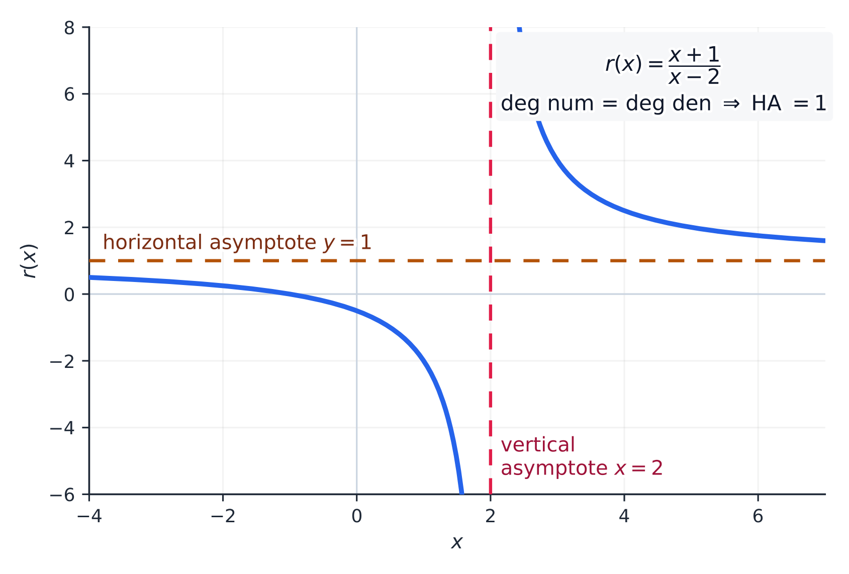
- Equal degrees: the quotient is a constant, giving a horizontal asymptote 水平渐近线 $y=$ the ratio of leading coefficients.
- Numerator degree < denominator degree: the quotient tends to $0$, so the horizontal asymptote is $y=0$.
At a horizontal asymptote $y=b$, the outputs get and stay arbitrarily close to $b$: $\lim_{x\to\pm\infty}r(x)=b$.
Vocabulary TrainEnglish rational function/ˈræʃənl ˈfʌŋkʃn/ slant asymptote/slænt ˈæsɪmptəʊt/ horizontal asymptote/ˌhɒrɪˈzɒntl ˈæsɪmptəʊt/ 1.8
Rational Functions and Zeros
Syllabus
Learning Objective Essential Knowledge 1.8.A
Determine the zeros of rational functions.- 1.8.A.1 The real zeros of a rational function correspond to the real zeros of the numerator for such values in its domain.
- 1.8.A.2 The real zeros of both polynomial functions of a rational function $r$ are endpoints or asymptotes for intervals satisfying the rational function inequalities $r(x) \geq 0$ or $r(x) \leq 0$.
Source: College Board AP Course and Exam Description
The real zeros of a rational function are the real zeros of its numerator that are still in the domain. These zeros, together with the zeros of the denominator, split the number line into the intervals you test when solving inequalities $r(x)\ge 0$ or $r(x)\le 0$.
1.9
Rational Functions and Vertical Asymptotes
Syllabus
Learning Objective Essential Knowledge 1.9.A
Determine vertical asymptotes of graphs of rational functions.- 1.9.A.1 If the value $a$ is a real zero of the polynomial function in the denominator of a rational function and is not also a real zero of the polynomial function in the numerator, then the graph of the rational function has a vertical asymptote at $x = a$. Furthermore, a vertical asymptote also occurs at $x = a$ if the multiplicity of $a$ as a real zero in the denominator is greater than its multiplicity as a real zero in the numerator.
- 1.9.A.2 Near a vertical asymptote, $x = a$, of a rational function, the values of the polynomial function in the denominator are arbitrarily close to zero, so the values of the rational function $r$ increase or decrease without bound. The corresponding mathematical notation is $\lim_{x \to a^+} r(x) = \infty$ or $\lim_{x \to a^+} r(x) = -\infty$ for input values near $a$ and greater than $a$, and $\lim_{x \to a^-} r(x) = \infty$ or $\lim_{x \to a^-} r(x) = -\infty$ for input values near $a$ and less than $a$.
Source: College Board AP Course and Exam Description
A vertical asymptote 垂直渐近线 occurs at $x=a$ when $a$ is a zero of the denominator but not cancelled by the numerator – more precisely, when its multiplicity in the denominator exceeds its multiplicity in the numerator. Near it, the denominator is nearly zero, so $r$ shoots to $\pm\infty$: $\lim_{x\to a^{\pm}}r(x)=\pm\infty$. Check each side, since the two sides can go opposite ways.
Worked example. Describe $r(x)=\dfrac{2x^2+3}{x^2-1}$. The numerator and denominator have equal degree, so the horizontal asymptote is $y=\dfrac{2}{1}=2$. The denominator $x^2-1$ is zero at $x=\pm1$ and neither cancels, so there are vertical asymptotes at $x=1$ and $x=-1$.
A rational function approaching a vertical asymptote and a horizontal asymptote ExploreExplore a vertical asymptote
y = a/(x − b) + c
This is $y = \dfrac{a}{x-b} + c$. The graph shoots off toward $\pm\infty$ at the vertical asymptote 竖直渐近线 $x = b$ (where the bottom is zero) and levels off toward the horizontal asymptote 水平渐近线 $y = c$. Slide $b$ and $c$ to move each line.
Vocabulary TrainEnglish vertical asymptote/ˈvɜːtɪkl ˈæsɪmptəʊt/ 1.10
Rational Functions and Holes
Syllabus
Learning Objective Essential Knowledge 1.10.A
Determine holes in graphs of rational functions.- 1.10.A.1 If the multiplicity of a real zero in the numerator is greater than or equal to its multiplicity in the denominator, then the graph of the rational function has a hole at the corresponding input value.
- 1.10.A.2 If the graph of a rational function $r$ has a hole at $x = c$, then the location of the hole can be determined by examining the output values corresponding to input values sufficiently close to $c$. If input values sufficiently close to $c$ correspond to output values arbitrarily close to $L$, then the hole is located at the point with coordinates $(c, L)$. The corresponding mathematical notation is $\lim_{x \to c} r(x) = L$. It should be noted that $\lim_{x \to c^-} r(x) = \lim_{x \to c^+} r(x) = \lim_{x \to c} r(x) = L$.
Source: College Board AP Course and Exam Description
A hole 空洞 (removable point) occurs at $x=c$ when a factor cancels – the multiplicity of the zero $c$ in the numerator is at least its multiplicity in the denominator. The graph is missing a single point. Its height is the limit of the simplified function: if inputs near $c$ give outputs near $L$, the hole is at $(c,L)$, and $\lim_{x\to c}r(x)=L$.
Vocabulary TrainEnglish hole/həʊl/ 1.11
Equivalent Representations of Polynomial and Rational Expressions
Syllabus
Learning Objective Essential Knowledge 1.11.A
Rewrite polynomial and rational expressions in equivalent forms.- 1.11.A.1 Because the factored form of a polynomial or rational function readily provides information about real zeros, it can reveal information about $x$-intercepts, asymptotes, holes, domain, and range.
- 1.11.A.2 The standard form of a polynomial or rational function can reveal information about end behaviors of the function.
- 1.11.A.3 The information extracted from different analytic representations of the same polynomial or rational function can be used to answer questions in context.
1.11.B
Determine the quotient of two polynomial functions using long division.- 1.11.B.1 Polynomial long division is an algebraic process similar to numerical long division involving a quotient and remainder. If the polynomial $f$ is divided by the polynomial $g$, then $f$ can be rewritten as $f(x) = g(x)q(x) + r(x)$, where $q$ is the quotient, $r$ is the remainder, and the degree of $r$ is less than the degree of $g$.
- 1.11.B.2 The result of polynomial long division is helpful in finding equations of slant asymptotes for graphs of rational functions.
1.11.C
Rewrite the repeated product of binomials using the binomial theorem.- 1.11.C.1 The binomial theorem utilizes the entries in a single row of Pascal's Triangle to more easily expand expressions of the form $(a + b)^n$, including polynomial functions of the form $p(x) = (x + c)^n$, where $c$ is a constant.
Source: College Board AP Course and Exam Description
The same expression, written differently, reveals different features:
- Factored form shows real zeros, and hence $x$-intercepts, holes, vertical asymptotes, and domain.
- Standard form (expanded) shows the degree and leading term, and hence end behavior.
Polynomial long division 多项式长除法 rewrites $f(x)=g(x)\,q(x)+r(x)$, where $q$ is the quotient 商 and $r$ the remainder 余数 (of smaller degree than $g$). The quotient gives the equation of a slant asymptote when the numerator's degree is one more than the denominator's.
Vocabulary TrainEnglish Polynomial long division/ˌpɒlɪˈnəʊmɪəl lɒŋ dɪˈvɪʒn/ quotient/ˈkwəʊʃənt/ remainder/rɪˈmeɪndə/ 1.12
Transformations of Functions
Syllabus
Learning Objective Essential Knowledge 1.12.A
Construct a function that is an additive and/or multiplicative transformation of another function.- 1.12.A.1 The function $g(x) = f(x) + k$ is an additive transformation of the function $f$ that results in a vertical translation of the graph of $f$ by $k$ units.
- 1.12.A.2 The function $g(x) = f(x + h)$ is an additive transformation of the function $f$ that results in a horizontal translation of the graph of $f$ by $-h$ units.
- 1.12.A.3 The function $g(x) = a f(x)$, where $a \neq 0$, is a multiplicative transformation of the function $f$ that results in a vertical dilation of the graph of $f$ by a factor of $|a|$. If $a < 0$, the transformation involves a reflection over the $x$-axis.
- 1.12.A.4 The function $g(x) = f(bx)$, where $b \neq 0$, is a multiplicative transformation of the function $f$ that results in a horizontal dilation of the graph of $f$ by a factor of $\left| \dfrac{1}{b} \right|$. If $b < 0$, the transformation involves a reflection over the $y$-axis.
- 1.12.A.5 Additive and multiplicative transformations can be combined, resulting in combinations of horizontal and vertical translations and dilations.
- 1.12.A.6 The domain and range of a function that is a transformation of a parent function may be different from those of the parent function.
Source: College Board AP Course and Exam Description
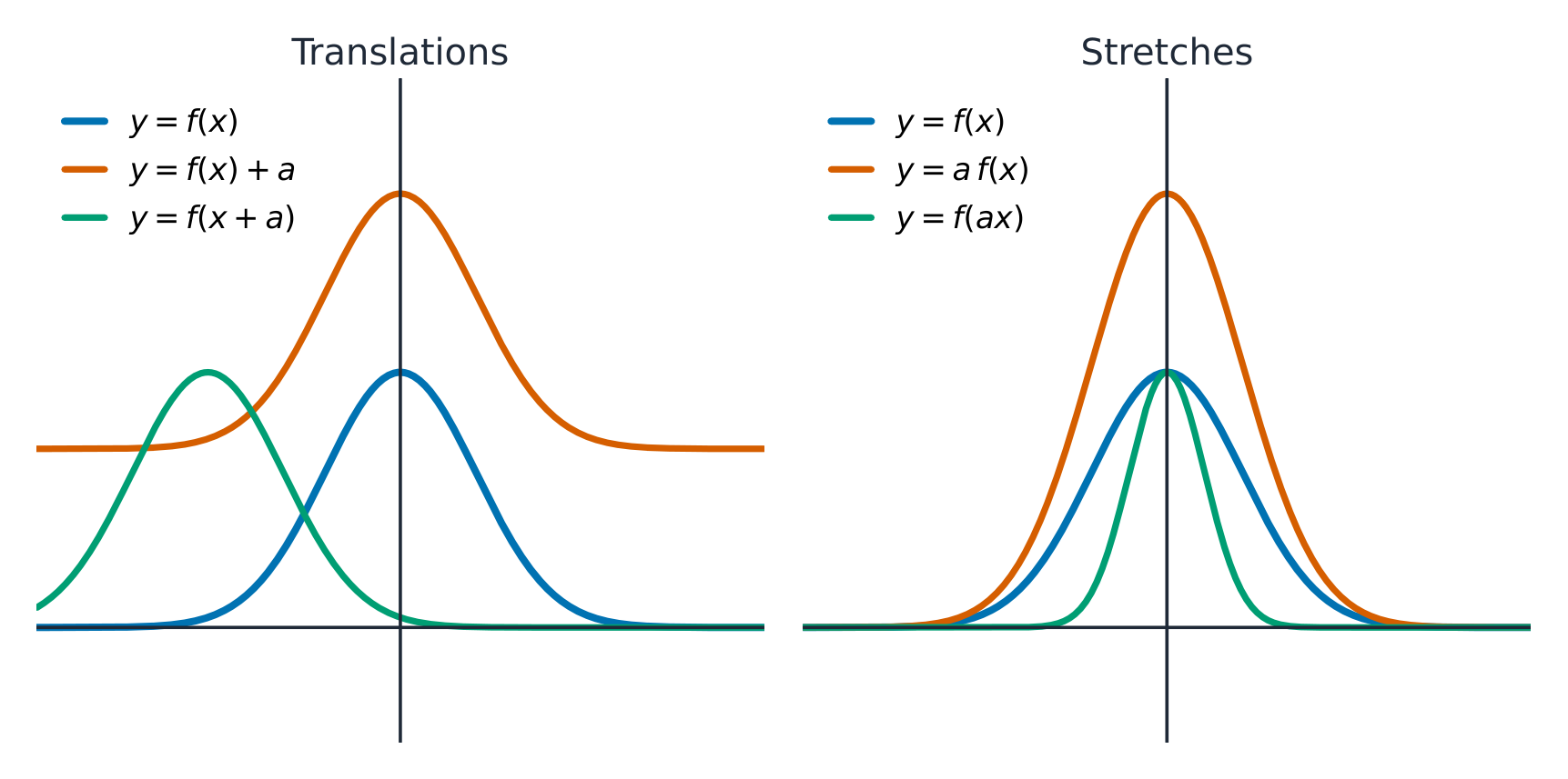
Transformations of graphs A transformation 变换 builds a new function from an old one $f$:
Adding to the output or input shifts the curve; a multiplier stretches it - Translations 平移 (shifts): $f(x)+k$ moves up/down; $f(x-h)$ moves right/left.
- Dilations 伸缩 (stretches): $a\,f(x)$ stretches vertically; $f(bx)$ stretches horizontally.
- Reflections 反射: $-f(x)$ flips over the $x$-axis; $f(-x)$ flips over the $y$-axis.
Combine additive shifts and multiplicative stretches to model shifted, scaled versions of a known shape.
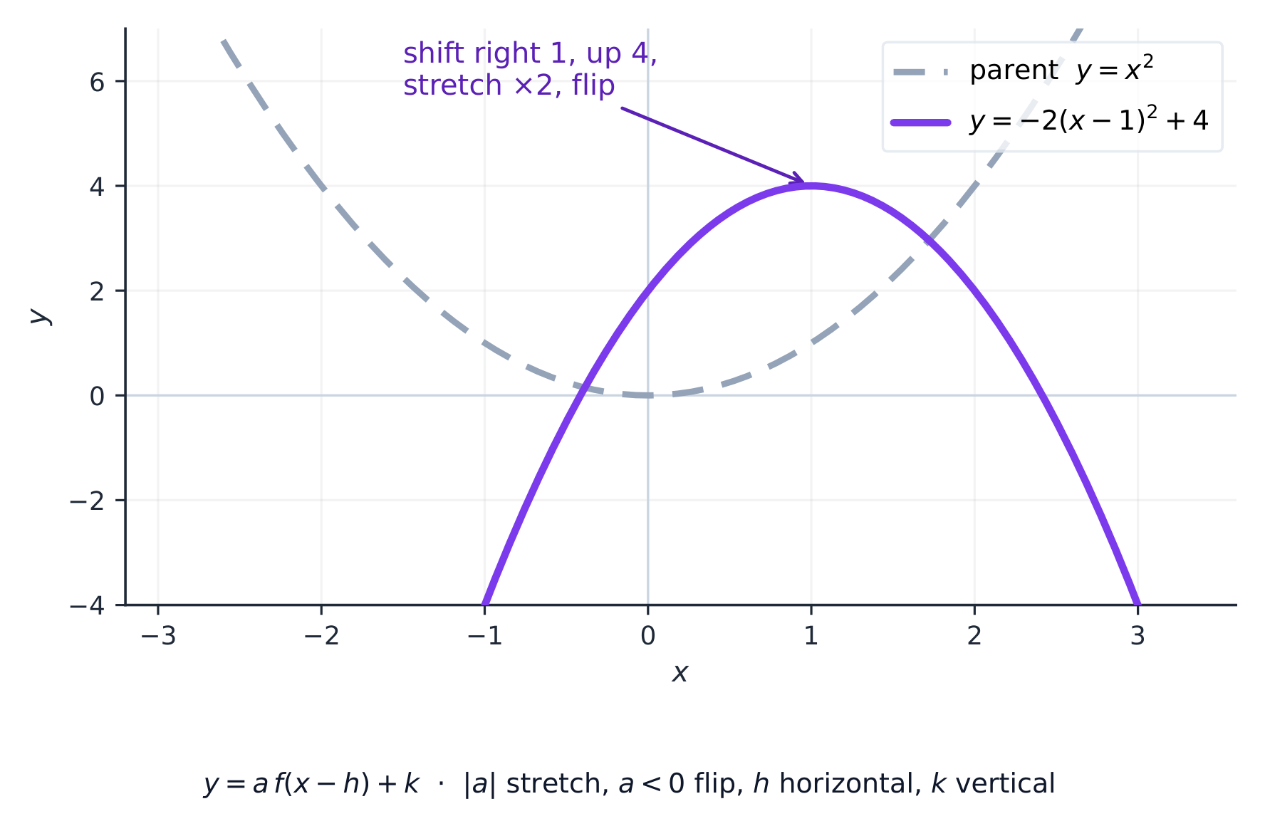
Transforming the parent parabola: shift, stretch, and reflect ExploreExplore shifts, stretches, and flips
Choose translate, reflect, rotate, or enlarge and change the amount. Watch which features stay the same — a transformation 变换 moves the whole graph without changing its underlying rule.
Vocabulary TrainEnglish transformation/trænsfɔːˈmeɪʃn/ Translations/trænˈsleɪʃnz/ Dilations/daɪˈleɪʃnz/ Reflections/rɪˈflekʃnz/ 1.13
Function Model Selection and Assumption Articulation
Syllabus
Learning Objective Essential Knowledge 1.13.A
Identify an appropriate function type to construct a function model for a given scenario.- 1.13.A.1 Linear functions model data sets or aspects of contextual scenarios that demonstrate roughly constant rates of change.
- 1.13.A.2 Quadratic functions model data sets or aspects of contextual scenarios that demonstrate roughly linear rates of change, or data sets that are roughly symmetric with a unique maximum or minimum value.
- 1.13.A.3 Geometric contexts involving area or two dimensions can often be modeled by quadratic functions. Geometric contexts involving volume or three dimensions can often be modeled by cubic functions.
- 1.13.A.4 Polynomial functions model data sets or contextual scenarios with multiple real zeros or multiple maxima or minima.
- 1.13.A.5 A polynomial function of degree $n$ models data sets or contextual scenarios that demonstrate roughly constant nonzero $n$th differences.
- 1.13.A.6 A polynomial function of degree $n$ or less can be used to model a graph of $n + 1$ points with distinct input values.
- 1.13.A.7 A piecewise-defined function consists of a set of functions defined over nonoverlapping domain intervals and is useful for modeling a data set or contextual scenario that demonstrates different characteristics over different intervals.
1.13.B
Describe assumptions and restrictions related to building a function model.- 1.13.B.1 A model may have underlying assumptions about what is consistent in the model.
- 1.13.B.2 A model may have underlying assumptions about how quantities change together.
- 1.13.B.3 A model may require domain restrictions based on mathematical clues, contextual clues, or extreme values in the data set.
- 1.13.B.4 A model may require range restrictions, such as rounding values, based on mathematical clues, contextual clues, or extreme values in the data set.
Source: College Board AP Course and Exam Description
Choosing a model 模型 means matching a function type to how a quantity changes. A linear model fits a constant rate of change; a quadratic fits a constant second difference; a polynomial fits data with several turns. In geometric situations the number of dimensions is a strong hint: quantities about area (two dimensions) are typically quadratic, and quantities about volume (three dimensions) are typically cubic – for example a box's volume as a function of a cut length. State the assumptions 假设 your model relies on (for example, that the pattern continues), because a model is only valid where those assumptions hold.
Vocabulary TrainEnglish model/ˈmɒdl/ assumptions/əˈsʌmpʃnz/ 1.14
Function Model Construction and Application
Syllabus
Learning Objective Essential Knowledge 1.14.A
Construct a linear, quadratic, cubic, quartic, polynomial of degree $n$, or related piecewise-defined function model.- 1.14.A.1 A model can be constructed based on restrictions identified in a mathematical or contextual scenario.
- 1.14.A.2 A model of a data set or a contextual scenario can be constructed using transformations of the parent function.
- 1.14.A.3 A model of a data set can be constructed using technology and regressions, including linear, quadratic, cubic, and quartic regressions.
- 1.14.A.4 A piecewise-defined function model can be constructed through a combination of modeling techniques.
1.14.B
Construct a rational function model based on a context.- 1.14.B.1 Data sets and aspects of contextual scenarios involving quantities that are inversely proportional can often be modeled by rational functions. For example, the magnitudes of both gravitational force and electromagnetic force between objects are inversely proportional to the objects' squared distance.
1.14.C
Apply a function model to answer questions about a data set or contextual scenario.- 1.14.C.1 A model can be used to draw conclusions about the modeled data set or contextual scenario, including answering key questions and predicting values, rates of change, average rates of change, and changing rates of change. Appropriate units of measure should be extracted or inferred from the given context.
Source: College Board AP Course and Exam Description
To construct a model, use given features – points, intercepts, zeros with multiplicities, end behavior – to write the function, then use it to answer questions in context. Always check the answer against the domain that makes sense for the situation, and interpret outputs with their real-world units.
A piecewise-defined function 分段函数 uses different rules over non-overlapping intervals of the domain. To evaluate it, pick the branch whose interval contains the input. For example,
$$f(x)=\begin{cases} x^2, & x<0\\ 2x, & x\ge 0\end{cases}$$gives $f(-3)=9$ from the first branch but $f(3)=6$ from the second – useful when behaviour changes at a threshold (a tiered price, a speed limit that changes).Vocabulary TrainEnglish piecewise-defined function/ˈpiːswaɪz dɪˈfaɪnd ˈfʌŋkʃn/ 1.14
Exam tips
- Read a function through its rate of change: average rate = secant slope; a constant rate means linear, a linear-changing rate means quadratic.
- Factor a polynomial to find zeros (x-intercepts) and their multiplicity; even multiplicity touches, odd crosses the axis.
- End behaviour is set by the leading term; a rational function's asymptotes come from the degrees of top and bottom.
- Build models from key features (points, zeros, end behaviour) and state your assumptions.
- Describe transformations precisely: shift $f(x-h)+k$, stretch $af(bx)$, reflect $-f(x)$ / $f(-x)$.
- increasing 递增 if, whenever $a
-
2
Exponential and Logarithmic Functions
Watch lesson2.1
Change in Arithmetic and Geometric Sequences
Syllabus
Learning Objective Essential Knowledge 2.1.A
Express arithmetic sequences found in mathematical and contextual scenarios as functions of the whole numbers.- 2.1.A.1 A sequence is a function from the whole numbers to the real numbers. Consequently, the graph of a sequence consists of discrete points instead of a curve.
- 2.1.A.2 Successive terms in an arithmetic sequence have a common difference, or constant rate of change.
- 2.1.A.3 The general term of an arithmetic sequence with a common difference $d$ is denoted by $a_n$ and is given by $a_n = a_0 + dn$, where $a_0$ is the initial value, or by $a_n = a_k + d(n - k)$, where $a_k$ is the $k$th term of the sequence.
2.1.B
Express geometric sequences found in mathematical and contextual scenarios as functions of the whole numbers.- 2.1.B.1 Successive terms in a geometric sequence have a common ratio, or constant proportional change.
- 2.1.B.2 The general term of a geometric sequence with a common ratio $r$ is denoted by $g_n$ and is given by $g_n = g_0 r^n$, where $g_0$ is the initial value, or by $g_n = g_k r^{(n-k)}$, where $g_k$ is the $k$th term of the sequence.
- 2.1.B.3 Increasing arithmetic sequences increase equally with each step, whereas increasing geometric sequences increase by a larger amount with each successive step.
Source: College Board AP Course and Exam Description
Geometric series & convergence A sequence 数列 is a function from the whole numbers to the real numbers, so its graph is discrete points, not a curve.
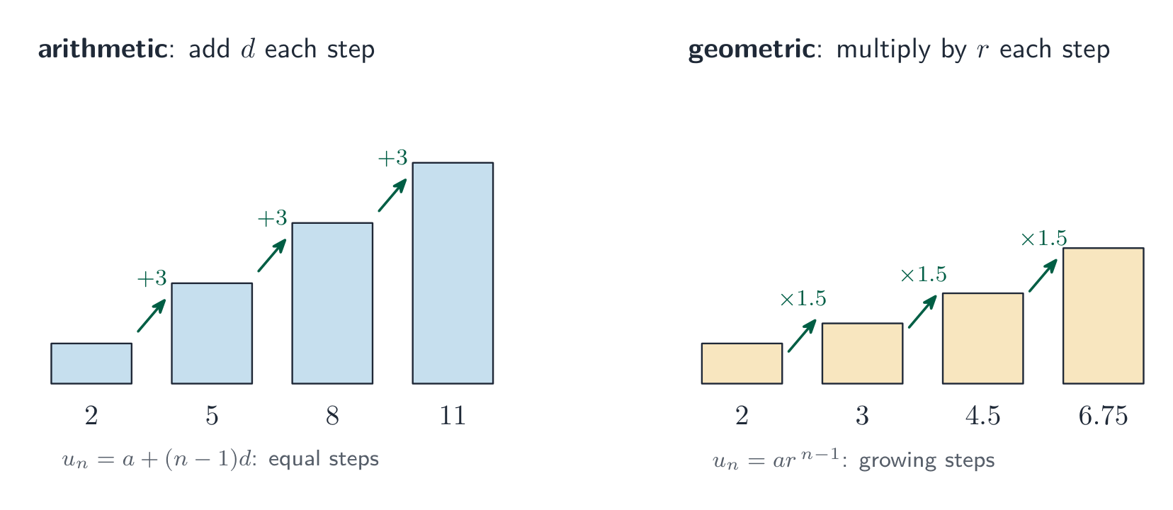
An arithmetic sequence climbs in equal steps; a geometric one multiplies by a ratio - An arithmetic sequence 等差数列 has a common difference 公差 $d$ (a constant rate of change): $a_n = a_0 + dn$, or from a known term, $a_n = a_k + d(n-k)$.
- A geometric sequence 等比数列 has a common ratio 公比 $r$ (a constant proportional change): $g_n = g_0\,r^{\,n}$, or $g_n = g_k\,r^{\,(n-k)}$.
An increasing arithmetic sequence grows by the same amount each step; an increasing geometric sequence grows by a larger amount each step.
Worked example. An arithmetic sequence with $a_0=3$ and $d=5$ has $a_4=3+5(4)=23$. A geometric sequence with $g_0=2$ and $r=3$ has $g_4=2\cdot3^4=162$ – addition versus multiplication makes the geometric one pull far ahead.
ExploreCompare arithmetic and geometric growth
An arithmetic sequence adds a fixed step each term (linear); a geometric sequence multiplies by a fixed ratio (exponential). Change the ratio and watch the terms explode or decay.
Vocabulary TrainEnglish sequence/ˈsiːkwəns/ arithmetic sequence/əˈrɪθmətɪk ˈsiːkwəns/ common difference/ˈkɒmən ˈdɪfrəns/ geometric sequence/ˌdʒiːəʊˈmetrɪk ˈsiːkwəns/ common ratio/ˈkɒmən ˈreɪʃɪəʊ/ 2.2
Change in Linear and Exponential Functions

Syllabus
Learning Objective Essential Knowledge 2.2.A
Construct functions of the real numbers that are comparable to arithmetic and geometric sequences.- 2.2.A.1 Linear functions of the form $f(x) = b + mx$ are similar to arithmetic sequences of the form $a_n = a_0 + dn$, as both can be expressed as an initial value ($b$ or $a_0$) plus repeated addition of a constant rate of change, the slope ($m$ or $d$).
- 2.2.A.2 Similar to arithmetic sequences of the form $a_n = a_k + d(n - k)$, which are based on a known difference, $d$, and a $k$th term, linear functions can be expressed in the form $f(x) = y_i + m(x - x_i)$ based on a known slope, $m$, and a point, $(x_i, y_i)$.
- 2.2.A.3 Exponential functions of the form $f(x) = ab^x$ are similar to geometric sequences of the form $g_n = g_0 r^n$, as both can be expressed as an initial value ($a$ or $g_0$) times repeated multiplication by a constant proportion ($b$ or $r$).
- 2.2.A.4 Similar to geometric sequences of the form $g_n = g_k r^{(n-k)}$, which are based on a known ratio, $r$, and a $k$th term, exponential functions can be expressed in the form $f(x) = y_i r^{(x - x_i)}$ based on a known ratio, $r$, and a point, $(x_i, y_i)$.
- 2.2.A.5 Sequences and their corresponding functions may have different domains.
Source: College Board AP Course and Exam Description
A sprinter: exponential and logarithmic models capture growth and decay rates in context Sequences have continuous cousins:
- Linear functions $f(x)=b+mx$ mirror arithmetic sequences – an initial value plus repeated addition of the slope $m$. Point form: $f(x)=y_i+m(x-x_i)$.
- Exponential functions $f(x)=ab^x$ mirror geometric sequences – an initial value times repeated multiplication by the base $b$. Point form: $f(x)=y_i\,r^{\,(x-x_i)}$.
The difference: linear = repeated addition, exponential = repeated multiplication. (A sequence and its function may have different domains.)
2.3
Exponential Functions
Syllabus
Learning Objective Essential Knowledge 2.3.A
Identify key characteristics of exponential functions.- 2.3.A.1 The general form of an exponential function is $f(x) = ab^x$, with the initial value $a$, where $a \neq 0$, and the base $b$, where $b > 0$, and $b \neq 1$. When $a > 0$ and $b > 1$, the exponential function is said to demonstrate exponential growth. When $a > 0$ and $0 < b < 1$, the exponential function is said to demonstrate exponential decay.
- 2.3.A.2 When the natural numbers are input values in an exponential function, the input value specifies the number of factors of the base to be applied to the function's initial value. The domain of an exponential function is all real numbers.
- 2.3.A.3 Because the output values of exponential functions in general form are proportional over equal-length input-value intervals, exponential functions are always increasing or always decreasing, and their graphs are always concave up or always concave down. Consequently, exponential functions do not have extrema except on a closed interval, and their graphs do not have points of inflection.
- 2.3.A.4 If the values of the additive transformation function $g(x) = f(x) + k$ of any function $f$ are proportional over equal-length input-value intervals, then $f$ is exponential.
Source: College Board AP Course and Exam Description
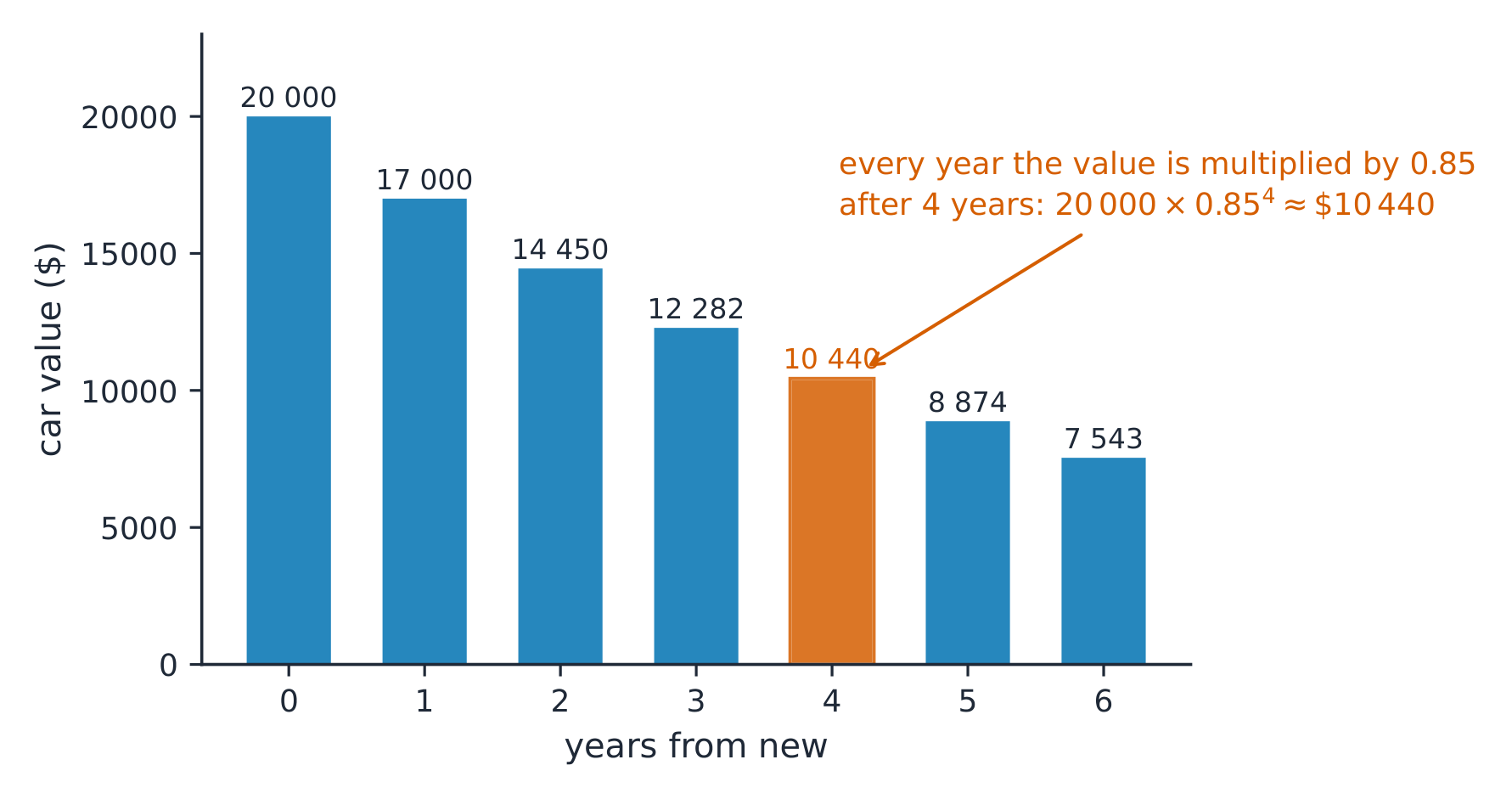
The general exponential function 指数函数 is $f(x)=ab^x$ with initial value 初始值 $a\neq 0$ and base 底数 $b>0,\ b\neq 1$. Domain: all real numbers.
Exponential decay: a fixed percentage is lost each period - $a>0,\ b>1$ gives exponential growth 指数增长; $a>0,\ 0
- Outputs are proportional over equal-length input intervals. So an exponential is always increasing or always decreasing, and always concave up or always concave down – it has no extrema (except on a closed interval) and no points of inflection.
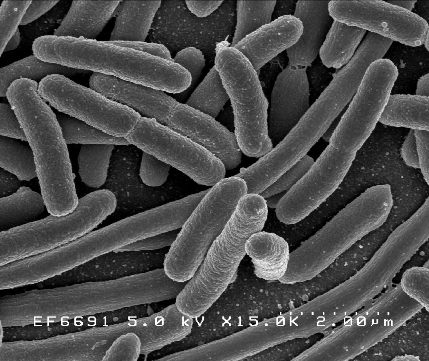
Bacteria under a microscope: exponential models describe populations that grow by a constant factor each time step ExploreExplore an exponential curve
y = a·e^(bx) + c
An exponential function changes by a constant factor over equal steps, so it rises (or decays) ever faster. The constant $c$ sets the horizontal asymptote it hugs.
Vocabulary TrainEnglish exponential function/ˌekspəˈnenʃl ˈfʌŋkʃn/ initial value/ɪˈnɪʃl ˈvæljuː/ base/beɪs/ exponential growth/ˌekspəˈnenʃl ɡrəʊθ/ exponential decay/ˌekspəˈnenʃl dɪˈkeɪ/ 2.4
Exponential Function Manipulation
Syllabus
Learning Objective Essential Knowledge 2.4.A
Rewrite exponential expressions in equivalent forms.- 2.4.A.1 The product property for exponents states that $b^m b^n = b^{(m+n)}$. Graphically, this property implies that every horizontal translation of an exponential function, $f(x) = b^{(x+k)}$, is equivalent to a vertical dilation, $f(x) = b^{(x+k)} = b^x b^k = ab^x$, where $a = b^k$.
- 2.4.A.2 The power property for exponents states that $\left(b^m\right)^n = b^{(mn)}$. Graphically, this property implies that every horizontal dilation of an exponential function, $f(x) = b^{(cx)}$, is equivalent to a change of the base of an exponential function, $f(x) = \left(b^c\right)^x$, where $b^c$ is a constant and $c \neq 0$.
- 2.4.A.3 The negative exponent property states that $b^{-n} = \dfrac{1}{b^n}$.
- 2.4.A.4 The value of an exponential expression involving an exponential unit fraction, such as $b^{(1/k)}$ where $k$ is a natural number, is the $k$th root of $b$, when it exists.
Source: College Board AP Course and Exam Description
The exponent rules reshape exponential expressions and connect to graph transformations:
- Product: $b^m b^n = b^{m+n}$. A horizontal shift $b^{x+k}$ equals a vertical stretch $ab^x$ with $a=b^k$.
- Power: $(b^m)^n = b^{mn}$. A horizontal stretch $b^{cx}$ equals a base change $(b^c)^x$.
- Negative exponent: $b^{-n}=\dfrac{1}{b^n}$.
- Unit-fraction exponent: $b^{1/k}=\sqrt[k]{b}$ (the $k$th root 方根).
Vocabulary TrainEnglish root/ruːt/ 2.5
Exponential Function Context and Data Modeling
Syllabus
Learning Objective Essential Knowledge 2.5.A
Construct a model for situations involving proportional output values over equal-length input-value intervals.- 2.5.A.1 Exponential functions model growth patterns where successive output values over equal-length input-value intervals are proportional. When the input values are whole numbers, exponential functions model situations of repeated multiplication of a constant to an initial value.
- 2.5.A.2 A constant may need to be added to the dependent variable values of a data set to reveal a proportional growth pattern.
- 2.5.A.3 An exponential function model can be constructed from an appropriate ratio and initial value or from two input-output pairs. The initial value and the base can be found by solving a system of equations resulting from the two input-output pairs.
- 2.5.A.4 Exponential function models can be constructed by applying transformations to $f(x) = ab^x$ based on characteristics of a contextual scenario or data set.
- 2.5.A.5 Exponential function models can be constructed for a data set with technology using exponential regressions.
- 2.5.A.6 The natural base $e$, which is approximately $2.718$, is often used as the base in exponential functions that model contextual scenarios.
Source: College Board AP Course and Exam Description
Exponentials model quantities that grow by a constant proportion over equal intervals (repeated multiplication).
- Build a model from a ratio and an initial value, or from two points (solve the system for $a$ and $b$).
- Sometimes a constant must be added to the data to reveal the proportional pattern.
- Use exponential regression 指数回归 on technology to fit a data set.
- The natural base 自然底数 $e\approx 2.718$ is the standard base for real-world models.
Vocabulary TrainEnglish exponential regression/ˌekspəˈnenʃl rɪˈɡreʃn/ natural base/ˈnætʃərəl beɪs/ 2.6
Competing Function Model Validation
Syllabus
Learning Objective Essential Knowledge 2.6.A
Construct linear, quadratic, and exponential models based on a data set.- 2.6.A.1 Two variables in a data set that demonstrate a slightly changing rate of change can be modeled by linear, quadratic, and exponential function models.
- 2.6.A.2 Models can be compared based on contextual clues and applicability to determine which model is most appropriate.
2.6.B
Validate a model constructed from a data set.- 2.6.B.1 A model is justified as appropriate for a data set if the graph of the residuals of a regression, the residual plot, appear without pattern.
- 2.6.B.2 The difference between the predicted and actual values is the error in the model. Depending on the data set and context, it may be more appropriate to have an underestimate or overestimate for any given interval.
Source: College Board AP Course and Exam Description
When a rate of change shifts only slightly, linear, quadratic, and exponential models may all seem to fit. Choose using context and fit quality:
- A model is appropriate if its residual plot 残差图 shows no pattern (a residual 残差 is actual minus predicted).
- The error is the gap between predicted and actual; context decides whether an over- or under-estimate is safer.
Vocabulary TrainEnglish residual plot/rɪˈsɪdʒuːəl plɒt/ residual/rɪˈsɪdʒuːəl/ 2.7
Composition of Functions

Syllabus
Learning Objective Essential Knowledge 2.7.A
Evaluate the composition of two or more functions for given values.- 2.7.A.1 If $f$ and $g$ are functions, the composite function $f \circ g$ maps a set of input values to a set of output values such that the output values of $g$ are used as input values of $f$. For this reason, the domain of the composite function is restricted to those input values of $g$ for which the corresponding output value is in the domain of $f$. $(f \circ g)(x)$ can also be represented as $f(g(x))$.
- 2.7.A.2 Values for the composite function $f \circ g$ can be calculated or estimated from the graphical, numerical, analytical, or verbal representations of $f$ and $g$ by using output values from $g$ as input values for $f$.
- 2.7.A.3 The composition of functions is not commutative; that is, $f \circ g$ and $g \circ f$ are typically different functions; therefore, $f(g(x))$ and $g(f(x))$ are typically different values.
- 2.7.A.4 If the function $f(x) = x$ is composed with any function $g$, the resulting composite function is the same as $g$; that is, $g(f(x)) = f(g(x)) = g(x)$. The function $f(x) = x$ is called the identity function. When composing two functions, the identify function acts in the same way as $0$, the additive identity, when adding two numbers and $1$, the multiplicative identity, when multiplying two numbers.
2.7.B
Construct a representation of the composition of two or more functions.- 2.7.B.1 Function composition is useful for relating two quantities that are not directly related by an existing formula.
- 2.7.B.2 When analytic representations of the functions $f$ and $g$ are available, an analytic representation of $f(g(x))$ can be constructed by substituting $g(x)$ for every instance of $x$ in $f$.
- 2.7.B.3 A numerical or graphical representation of $f \circ g$ can often be constructed by calculating or estimating values for $(x, f(g(x)))$.
2.7.C
Rewrite a given function as a composition of two or more functions.- 2.7.C.1 Functions given analytically can often be decomposed into less complicated functions. When properly decomposed, the variable in one function should replace each instance of the function with which it was composed.
- 2.7.C.2 An additive transformation of a function, $f$, that results in vertical and horizontal translations can be understood as the composition of $g(x) = x + k$ with $f$.
- 2.7.C.3 A multiplicative transformation of a function, $f$, that results in vertical and horizontal dilations can be understood as the composition of $g(x) = kx$ with $f$.
Source: College Board AP Course and Exam Description
The composite function 复合函数 $(f\circ g)(x)=f(g(x))$ feeds $g$'s output into $f$. Its domain is the inputs of $g$ whose outputs lie in $f$'s domain.
A function as a machine; its inverse runs the machine backwards - Composition is not commutative: $f(g(x))$ and $g(f(x))$ usually differ.
- To build $f(g(x))$ analytically, substitute $g(x)$ for every $x$ in $f$.
- The identity function 恒等函数 $f(x)=x$ leaves any function unchanged under composition.
- A function can also be decomposed into simpler pieces – useful for seeing an additive shift as composing with $x+k$, or a dilation as composing with $kx$.

Matryoshka dolls: function composition nests layers — evaluate the inside first Vocabulary TrainEnglish composite function/ˈkɒmpəzɪt ˈfʌŋkʃn/ identity function/aɪˈdentɪti ˈfʌŋkʃn/ 2.8
Inverse Functions
Syllabus
Learning Objective Essential Knowledge 2.8.A
Determine the input-output pairs of the inverse of a function.- 2.8.A.1 On a specified domain, a function, $f$, has an inverse function, or is invertible, if each output value of $f$ is mapped from a unique input value. The domain of a function may be restricted in many ways to make the function invertible.
- 2.8.A.2 An inverse function can be thought of as a reverse mapping of the function. An inverse function, $f^{-1}$, maps the output values of a function, $f$, on its invertible domain to their corresponding input values; that is, if $f(a) = b$, then $f^{-1}(b) = a$. Alternately, on its invertible domain, if a function consists of input-output pairs $(a, b)$, then the inverse function consists of input-output pairs $(b, a)$.
2.8.B
Determine the inverse of a function on an invertible domain.- 2.8.B.1 The composition of a function, $f$, and its inverse function, $f^{-1}$, is the identity function; that is, $f\left(f^{-1}(x)\right) = f^{-1}(f(x)) = x$.
- 2.8.B.2 On a function's invertible domain, the function's range and domain are the inverse function's domain and range, respectively. The inverse of the table of values of $y = f(x)$ can be found by reversing the input-output pairs; that is, $(a, b)$ corresponds to $(b, a)$.
- 2.8.B.3 The inverse of the graph of the function $y = f(x)$ can be found by reversing the roles of the $x$- and $y$-axes; that is, by reflecting the graph of the function over the graph of the identity function $h(x) = x$.
- 2.8.B.4 The inverse of the function can be found by determining the inverse operations to reverse the mapping. One method for finding the inverse of the function $f$ is reversing the roles of $x$ and $y$ in the equation $y = f(x)$, then solving for $y = f^{-1}(x)$.
- 2.8.B.5 In addition to limiting the domain of a function to obtain an inverse function, contextual restrictions may also limit the applicability of an inverse function.
Source: College Board AP Course and Exam Description
Inverse functions are a reflection Exponential & logarithm are inverses A function is invertible 可逆 on a domain where each output comes from a unique input (you may restrict the domain to force this). The inverse function 反函数 $f^{-1}$ reverses the mapping: if $f(a)=b$ then $f^{-1}(b)=a$.
- $f\big(f^{-1}(x)\big)=f^{-1}\big(f(x)\big)=x$ (composition gives the identity).
- Domain and range swap: reverse each $(a,b)$ to $(b,a)$ in a table; reflect the graph over the line $y=x$.
- To find a formula: swap $x$ and $y$ in $y=f(x)$, then solve for $y$. Context may further limit where the inverse applies.
Vocabulary TrainEnglish invertible/ɪnˈvɜːtɪbl/ inverse function/ɪnˈvɜːs ˈfʌŋkʃn/ 2.9
Logarithmic Expressions
Syllabus
Learning Objective Essential Knowledge 2.9.A
Evaluate logarithmic expressions.- 2.9.A.1 The logarithmic expression $\log_b c$ is equal to, or represents, the value that the base $b$ must be exponentially raised to in order to obtain the value $c$. That is, $\log_b c = a$ if and only if $b^a = c$, where $a$ and $c$ are constants, $b > 0$, and $b \neq 1$. (when the base of a logarithmic expression is not specified, it is understood as the common logarithm with a base of $10$)
- 2.9.A.2 The values of some logarithmic expressions are readily accessible through basic arithmetic while other values can be estimated through the use of technology.
- 2.9.A.3 On a logarithmic scale, each unit represents a multiplicative change of the base of the logarithm. For example, on a standard scale, the units might be $0, \; 1, \; 2, \; \ldots$, while on a logarithmic scale, using logarithm base $10$, the units might be $10^0, \; 10^1, \; 10^2, \; \ldots$.
Source: College Board AP Course and Exam Description
The logarithm 对数 answers "what exponent?": $\log_b c = a$ means exactly $b^a = c$ (with $b>0,\ b\neq 1$). An unwritten base means the common logarithm 常用对数 (base $10$). On a logarithmic scale, each unit is a multiplicative step of the base (…, $10^0,10^1,10^2,$ …).
Vocabulary TrainEnglish logarithm/ˈlɒɡərɪθəm/ common logarithm/ˈkɒmən ˈlɒɡərɪθəm/ 2.10
Inverses of Exponential Functions
Syllabus
Learning Objective Essential Knowledge 2.10.A
Construct representations of the inverse of an exponential function with an initial value of 1.- 2.10.A.1 The general form of a logarithmic function is $f(x) = a\log_b x$, with base $b$, where $b > 0$, $b \neq 1$, and $a \neq 0$.
- 2.10.A.2 The way in which input and output values vary together have an inverse relationship in exponential and logarithmic functions. Output values of general-form exponential functions change proportionately as input values increase in equal-length intervals. However, input values of general-form logarithmic functions change proportionately as output values increase in equal-length intervals. Alternately, exponential growth is characterized by output values changing multiplicatively as input values change additively, whereas logarithmic growth is characterized by output values changing additively as input values change multiplicatively.
- 2.10.A.3 $f(x) = \log_b x$ and $g(x) = b^x$, where $b > 0$ and $b \neq 1$, are inverse functions. That is, $g(f(x)) = f(g(x)) = x$.
- 2.10.A.4 The graph of the logarithmic function $f(x) = \log_b x$, where $b > 0$ and $b \neq 1$, is a reflection of the graph of the exponential function $g(x) = b^x$, where $b > 0$ and $b \neq 1$, over the graph of the identity function $h(x) = x$.
- 2.10.A.5 If $(s, \; t)$ is an ordered pair of the exponential function $g(x) = b^x$, where $b > 0$ and $b \neq 1$, then $(t, \; s)$ is an ordered pair of the logarithmic function $f(x) = \log_b x$, where $b > 0$ and $b \neq 1$.
Source: College Board AP Course and Exam Description
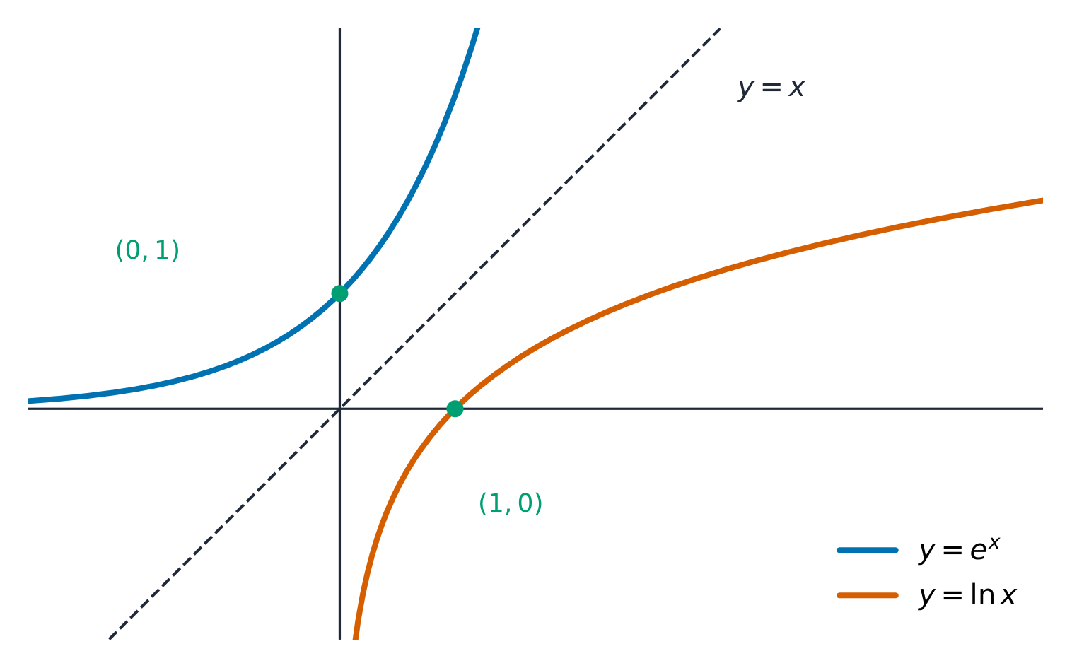
The logarithm is the inverse of the exponential: $y=b^x$ and $y=\log_b x$ undo each other, so their graphs are reflections over $y=x$. Hence $\log_b(b^x)=x$ and $b^{\log_b x}=x$. The natural logarithm 自然对数 $\ln x = \log_e x$ is the inverse of $e^x$.
e^x and ln x are reflections of each other in the line y = x Vocabulary TrainEnglish natural logarithm/ˈnætʃərəl ˈlɒɡərɪθəm/ 2.11
Logarithmic Functions
Syllabus
Learning Objective Essential Knowledge 2.11.A
Identify key characteristics of logarithmic functions.- 2.11.A.1 The domain of a logarithmic function in general form is any real number greater than zero, and its range is all real numbers.
- 2.11.A.2 Because logarithmic functions are inverses of exponential functions, logarithmic functions are also always increasing or always decreasing, and their graphs are either always concave up or always concave down. Consequently, logarithmic functions do not have extrema except on a closed interval, and their graphs do not have points of inflection.
- 2.11.A.3 The additive transformation function $g(x) = f(x + k)$, where $k \neq 0$, of a logarithmic function $f$ in general form does not have input values that are proportional over equal-length output-value intervals. However, if the input values of the additive transformation function, $g(x) = f(x + k)$, of any function $f$ are proportional over equal-length output value intervals, then $f$ is logarithmic.
- 2.11.A.4 With their limited domain, logarithmic functions in general form are vertically asymptotic to $x = 0$, with an end behavior that is unbounded. That is, for a logarithmic function in general form, $\lim\limits_{x \to 0^+} a\log_b x = \pm\infty$ and $\lim\limits_{x \to \infty} a\log_b x = \pm\infty$.
Source: College Board AP Course and Exam Description
The logarithmic function 对数函数 $f(x)=\log_b x$ has domain $x>0$ and range all reals. It is always increasing (for $b>1$) or always decreasing (for $0
ExploreExplore a logarithmic curve
y = a·ln(x − b) + c
A logarithm is the inverse of an exponential: it grows without bound but ever slower, with a vertical asymptote where its input hits zero.
Vocabulary TrainEnglish logarithmic function/ˌlɒɡəˈrɪθmɪk ˈfʌŋkʃn/ 2.12
Logarithmic Function Manipulation
Syllabus
Learning Objective Essential Knowledge 2.12.A
Rewrite logarithmic expressions in equivalent forms.- 2.12.A.1 The product property for logarithms states that $\log_b(xy) = \log_b x + \log_b y$. Graphically, this property implies that every horizontal dilation of a logarithmic function, $f(x) = \log_b(kx)$, is equivalent to a vertical translation, $f(x) = \log_b(kx) = \log_b k + \log_b x = a + \log_b x$, where $a = \log_b k$.
- 2.12.A.2 The power property for logarithms states that $\log_b x^n = n\log_b x$. Graphically, this property implies that raising the input of a logarithmic function to a power, $f(x) = \log_b x^k$, results in a vertical dilation, $f(x) = \log_b x^k = k\log_b x$.
- 2.12.A.3 The change of base property for logarithms states that $\log_b x = \dfrac{\log_a x}{\log_a b}$, where $a > 0$ and $a \neq 1$. This implies that all logarithmic functions are vertical dilations of each other.
- 2.12.A.4 The function $f(x) = \ln x$ is a logarithmic function with the natural base $e$; that is, $\ln x = \log_e x$.
Source: College Board AP Course and Exam Description
The log properties reverse the exponent rules:
$$\log_b(xy)=\log_b x+\log_b y,\quad \log_b\!\frac{x}{y}=\log_b x-\log_b y,\quad \log_b(x^n)=n\log_b x.$$The change-of-base 换底 formula lets you compute any log with technology: $\log_b x = \dfrac{\log x}{\log b}=\dfrac{\ln x}{\ln b}$.Vocabulary TrainEnglish change-of-base/tʃeɪndʒ ɒv beɪs/ 2.13
Exponential and Logarithmic Equations and Inequalities
Syllabus
Learning Objective Essential Knowledge 2.13.A
Solve exponential and logarithmic equations and inequalities.- 2.13.A.1 Properties of exponents, properties of logarithms, and the inverse relationship between exponential and logarithmic functions can be used to solve equations and inequalities involving exponents and logarithms.
- 2.13.A.2 When solving exponential and logarithmic equations found through analytical or graphical methods, the results should be examined for extraneous solutions precluded by the mathematical or contextual limitations.
- 2.13.A.3 Logarithms can be used to rewrite expressions involving exponential functions in different ways that may reveal helpful information. Specifically, $b^x = c^{(\log_c b)(x)}$.
2.13.B
Construct the inverse function for exponential and logarithmic functions.- 2.13.B.1 The function $f(x) = ab^{(x-h)} + k$ is a combination of additive transformations of an exponential function in general form. The inverse of $y = f(x)$ can be found by determining the inverse operations to reverse the mapping.
- 2.13.B.2 The function $f(x) = a\log_b(x - h) + k$ is a combination of additive transformations of a logarithmic function in general form. The inverse of $y = f(x)$ can be found by determining the inverse operations to reverse the mapping.
Source: College Board AP Course and Exam Description
To solve, use the fact that exponentials and logs are inverses:
- Isolate the exponential, then take a log of both sides (bring the exponent down with the power property).
- Isolate the log, then exponentiate both sides.
- Always check for extraneous solutions – the argument of a log must stay positive.
Worked example. Solve $2\cdot3^x=54$. Divide by $2$: $3^x=27=3^3$, so $x=3$. When the sides are not tidy powers, take logs instead: $5^x=20$ gives $x=\dfrac{\ln 20}{\ln 5}\approx1.86$.
2.14
Logarithmic Function Context and Data Modeling
Syllabus
Learning Objective Essential Knowledge 2.14.A
Construct a logarithmic function model.- 2.14.A.1 Logarithmic functions are inverses of exponential functions and can be used to model situations involving proportional growth, or repeated multiplication, where the input values change proportionally over equal-length output-value intervals. Alternately, if the output value is a whole number, it indicates how many times the initial value has been multiplied by the proportion.
- 2.14.A.2 A logarithmic function model can be constructed from an appropriate proportion and a real zero or from two input-output pairs.
- 2.14.A.3 Logarithmic function models can be constructed by applying transformations to $f(x) = a\log_b x$ based on characteristics of a context or data set.
- 2.14.A.4 Logarithmic function models can be constructed for a data set with technology using logarithmic regressions.
- 2.14.A.5 The natural logarithm function is often useful in modeling real-world phenomena.
- 2.14.A.6 Logarithmic function models can be used to predict values for the dependent variable.
Source: College Board AP Course and Exam Description
Logarithms model quantities that change over huge multiplicative ranges (sound, acid strength, earthquakes). Build a log model from data, and use logarithmic regression for a data set. Because a log compresses large values, it turns proportional growth into a straight-line pattern – the idea behind semi-log plots.
2.15
Semi-log Plots
Syllabus
Learning Objective Essential Knowledge 2.15.A
Determine if an exponential model is appropriate by examining a semi-log plot of a data set.- 2.15.A.1 In a semi-log plot, one of the axes is logarithmically scaled. When the $y$-axis of a semi-log plot is logarithmically scaled, data or functions that demonstrate exponential characteristics will appear linear.
- 2.15.A.2 An advantage of semi-log plots is that a constant never needs to be added to the dependent variable values to reveal that an exponential model is appropriate.
2.15.B
Construct the linearization of exponential data.- 2.15.B.1 Techniques used to model linear functions can be applied to a semi-log graph.
- 2.15.B.2 For an exponential model of the form $y = ab^x$, the corresponding linear model for the semi-log plot is $y = (\log_n b)x + \log_n a$, where $n > 0$ and $n \neq 1$. Specifically, the linear rate of change is $\log_n b$, and the initial linear value is $\log_n a$.
Source: College Board AP Course and Exam Description
A semi-log plot 半对数图 puts the output on a logarithmic axis and the input on a normal axis. On these axes, an exponential function $y=ab^x$ becomes a straight line, because $\log y = \log a + (\log b)\,x$ is linear in $x$. So: if data look linear on a semi-log plot, an exponential model fits; the line's slope gives $\log b$ and its intercept gives $\log a$.
Vocabulary TrainEnglish semi-log plot/ˈsemi lɒɡ plɒt/ 2.15
Exam tips
- Distinguish arithmetic (add a common difference) from geometric (multiply a common ratio) sequences and their linear/exponential function cousins.
- Exponential = repeated multiplication, so it eventually outgrows any linear or polynomial model.
- The logarithm is the inverse of the exponential ($\log_b c=a\Leftrightarrow b^a=c$); use it to solve $b^x=k$.
- Apply the log laws (product, quotient, power) and the change-of-base formula; the argument of a log must be positive.
- On a semi-log plot an exponential model becomes a straight line.
-
3
Trigonometric and Polar Functions
Watch lesson3.1
Periodic Phenomena

Syllabus
Learning Objective Essential Knowledge 3.1.A
Construct graphs of periodic relationships based on verbal representations.- 3.1.A.1 A periodic relationship can be identified between two aspects of a context if, as the input values increase, the output values demonstrate a repeating pattern over successive equal-length intervals.
- 3.1.A.2 The graph of a periodic relationship can be constructed from the graph of a single cycle of the relationship.
3.1.B
Describe key characteristics of a periodic function based on a verbal representation.- 3.1.B.1 The period of the function is the smallest positive value $k$ such that $f(x + k) = f(x)$ for all $x$ in the domain. Consequently, the behavior of a periodic function is completely determined by any interval of width $k$.
- 3.1.B.2 The period can be estimated by investigating successive equal-length output values and finding where the pattern begins to repeat.
- 3.1.B.3 Periodic functions take on characteristics of other functions, such as intervals of increase and decrease, different concavities, and various rates of change. However, with periodic functions, all characteristics found in one period of the function will be in every period of the function.
Source: College Board AP Course and Exam Description
The ISS in orbit: trigonometric and polar functions describe periodic and circular motion A relationship is periodic 周期性 if its output pattern repeats at regular input steps. The period 周期 is the smallest positive $k$ with $f(x+k)=f(x)$ for all $x$. You can build the whole graph by copying a single cycle 周期段, and estimate the period by finding how far apart the pattern repeats. Within each cycle a periodic function still has intervals of increase/decrease and maxima/minima.
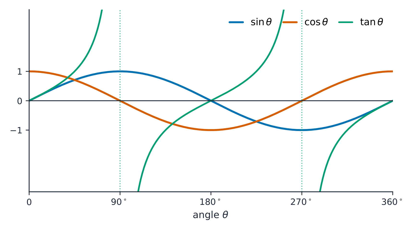
sin and cos wave between -1 and 1; tan breaks at 90 and 270 degrees 
As a Ferris wheel turns steadily, your height rises and falls over and over — a real sine wave in time Vocabulary TrainEnglish periodic/ˌpɪərɪˈɒdɪk/ period/ˈpɪərɪəd/ cycle/ˈsaɪkl/ 3.2
Sine, Cosine, and Tangent
Syllabus
Learning Objective Essential Knowledge 3.2.A
Determine the sine, cosine, and tangent of an angle using the unit circle.- 3.2.A.1 In the coordinate plane, an angle is in standard position when the vertex coincides with the origin and one ray coincides with the positive $x$-axis. The other ray is called the terminal ray. Positive and negative angle measures indicate rotations from the positive $x$-axis in the counterclockwise and clockwise direction, respectively. Angles in standard position that share a terminal ray differ by an integer number of revolutions.
- 3.2.A.2 The radian measure of an angle in standard position is the ratio of the length of the arc of a circle centered at the origin subtended by the angle to the radius of that same circle. For a unit circle, which has radius $1$, the radian measure is the same as the length of the subtended arc.
- 3.2.A.3 Given an angle in standard position and a circle centered at the origin, there is a point, $P$, where the terminal ray intersects the circle. The sine of the angle is the ratio of the vertical displacement of $P$ from the $x$-axis to the distance between the origin and point $P$. Therefore, for a unit circle, the sine of the angle is the $y$-coordinate of point $P$.
- 3.2.A.4 Given an angle in standard position and a circle centered at the origin, there is a point, $P$, where the terminal ray intersects the circle. The cosine of the angle is the ratio of the horizontal displacement of $P$ from the $y$-axis to the distance between the origin and point $P$. Therefore, for a unit circle, the cosine of the angle is the $x$-coordinate of point $P$.
- 3.2.A.5 Given an angle in standard position, the tangent of the angle is the slope, if it exists, of the terminal ray. Because the slope of the terminal ray is the ratio of the vertical displacement to the horizontal displacement over any interval, the tangent of the angle is the ratio of the $y$-coordinate to the $x$-coordinate of the point at which the terminal ray intersects the unit circle; alternately, it is the ratio of the angle's sine to its cosine.
Source: College Board AP Course and Exam Description
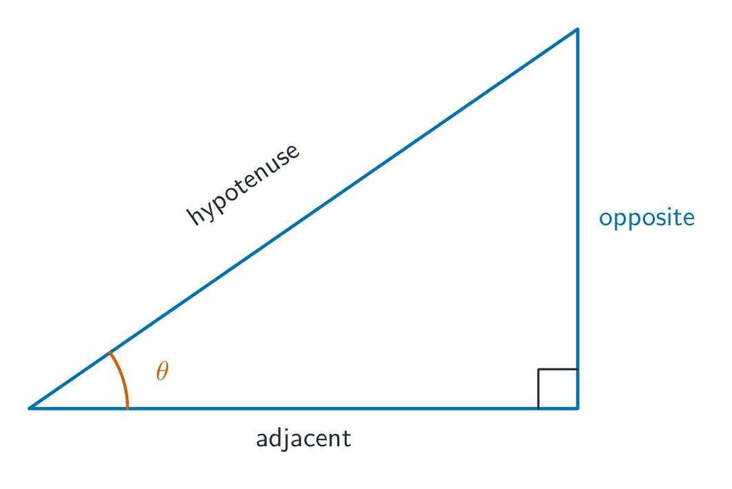
An angle is in standard position 标准位置 when its vertex is at the origin and its initial ray lies on the positive $x$-axis. Its radian 弧度 measure is the arc length on a unit circle. For the point $P$ where the terminal ray meets a circle of radius $r$:
$$\cos\theta = \frac{x}{r},\qquad \sin\theta = \frac{y}{r},\qquad \tan\theta = \frac{y}{x}\ (\text{the slope of the terminal ray}).$$Naming the sides of a right triangle from the angle ExploreRead sine and cosine off the unit circle
On the unit circle a point at angle $\theta$ has coordinates $(\cos\theta,\ \sin\theta)$. Spin the angle to watch sine and cosine trace out as the height and width.
Vocabulary TrainEnglish standard position/ˈstændəd pəˈzɪʃn/ radian/ˈreɪdɪən/ 3.3
Sine and Cosine Function Values
Syllabus
Learning Objective Essential Knowledge 3.3.A
Determine coordinates of points on a circle centered at the origin.- 3.3.A.1 Given an angle of measure $\theta$ in standard position and a circle with radius $r$ centered at the origin, there is a point, $P$, where the terminal ray intersects the circle. The coordinates of point $P$ are $(r\cos\theta, r\sin\theta)$.
- 3.3.A.2 The geometry of isosceles right and equilateral triangles, while attending to the signs of the values based on the quadrant of the angle, can be used to find exact values for the cosine and sine of angles that are multiples of $\dfrac{\pi}{4}$ and $\dfrac{\pi}{6}$ radians and whose terminal rays do not lie on an axis.
Source: College Board AP Course and Exam Description
On a circle of radius $r$, $x=r\cos\theta$ and $y=r\sin\theta$. Exact values at the special angles ($0,\tfrac{\pi}{6},\tfrac{\pi}{4},\tfrac{\pi}{3},\tfrac{\pi}{2},\dots$) come from isosceles right and equilateral triangle 等边三角形 geometry, with signs set by the quadrant 象限 of the angle.
Vocabulary TrainEnglish equilateral triangle/ˌiːkwɪˈlætərəl ˈtraɪæŋɡl/ quadrant/ˈkwɒdrənt/ 3.4
Sine and Cosine Function Graphs
Syllabus
Learning Objective Essential Knowledge 3.4.A
Construct representations of the sine and cosine functions using the unit circle.- 3.4.A.1 Given an angle of measure $\theta$ in standard position and a unit circle centered at the origin, there is a point, $P$, where the terminal ray intersects the circle. The sine function, $f(\theta) = \sin\theta$, gives the $y$-coordinate, or vertical displacement from the $x$-axis, of point $P$. The domain of the sine function is all real numbers.
- 3.4.A.2 As the input values, or angle measures, of the sine function increase, the output values oscillate between $-1$ and $1$, taking every value in between and tracking the vertical distance of points on the unit circle from the $x$-axis.
- 3.4.A.3 Given an angle of measure $\theta$ in standard position and a unit circle centered at the origin, there is a point, $P$, where the terminal ray intersects the circle. The cosine function, $f(\theta) = \cos\theta$, gives the $x$-coordinate, or horizontal displacement from the $y$-axis, of point $P$. The domain of the cosine function is all real numbers.
- 3.4.A.4 As the input values, or angle measures, of the cosine function increase, the output values oscillate between $-1$ and $1$, taking every value in between and tracking the horizontal distance of points on the unit circle from the $y$-axis.
Source: College Board AP Course and Exam Description
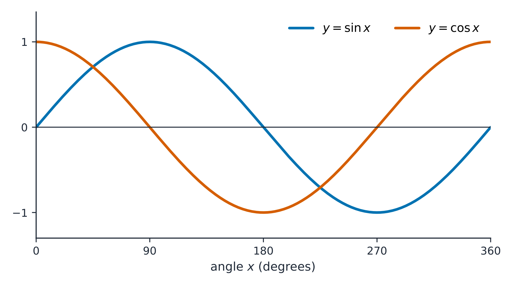
The unit circle draws the sine curve On the unit circle 单位圆 ($r=1$), $\sin\theta$ is the $y$-coordinate and $\cos\theta$ is the $x$-coordinate. As $\theta$ increases, both oscillate 振荡 smoothly between $-1$ and $1$ with period $2\pi$. Sine starts at $0$ (rising); cosine starts at $1$. They are the same wave shifted by $\tfrac{\pi}{2}$.
y = sin x and y = cos x are smooth waves between -1 and 1 ExploreGraph a sine wave
Unrolling the circle gives the wave $y=\sin x$: it repeats every $2\pi$ (its period) and swings between $-1$ and $1$ (its amplitude).
Vocabulary TrainEnglish unit circle/ˈjuːnɪt ˈsɜːkl/ oscillate/ˈɒsɪleɪt/ 3.5
Sinusoidal Functions
Syllabus
Learning Objective Essential Knowledge 3.5.A
Identify key characteristics of the sine and cosine functions.- 3.5.A.1 A sinusoidal function is any function that involves additive and multiplicative transformations of $f(\theta) = \sin\theta$. The sine and cosine functions are both sinusoidal functions, with $\cos\theta = \sin\left(\theta + \dfrac{\pi}{2}\right)$.
- 3.5.A.2 The period and frequency of a sinusoidal function are reciprocals. The period of $f(\theta) = \sin\theta$ and $g(\theta) = \cos\theta$ is $2\pi$, and the frequency is $\dfrac{1}{2\pi}$.
- 3.5.A.3 The amplitude of a sinusoidal function is half the difference between its maximum and minimum values. The amplitude of $f(\theta) = \sin\theta$ and $g(\theta) = \cos\theta$ is $1$.
- 3.5.A.4 The midline of the graph of a sinusoidal function is determined by the average, or arithmetic mean, of the maximum and minimum values of the function. The midline of the graphs of $y = \sin\theta$ and $y = \cos\theta$ is $y = 0$.
- 3.5.A.5 As input values increase, the graphs of sinusoidal functions oscillate between concave down and concave up.
- 3.5.A.6 The graph of $y = \sin\theta$ has rotational symmetry about the origin and is therefore an odd function. The graph of $y = \cos\theta$ has reflective symmetry over the $y$-axis and is therefore an even function.
Source: College Board AP Course and Exam Description
A sinusoidal function 正弦型函数 is any transformation of sine (or cosine). Its key features:
- Period and frequency 频率 are reciprocals; $\sin\theta$ has period $2\pi$.
- Amplitude 振幅 = half the distance between the maximum and minimum output.
- Midline 中线 $y=d$ = the average of the maximum and minimum (the horizontal center line).
The graph alternates concave up and concave down each half-cycle.
Worked example. For $f(\theta)=3\sin(2\theta)+1$: the amplitude is $3$, the period is $\dfrac{2\pi}{2}=\pi$, and the midline is $y=1$. So the maximum output is $1+3=4$ and the minimum is $1-3=-2$.
Vocabulary TrainEnglish sinusoidal function/ˌsaɪnəˈsɔɪdl ˈfʌŋkʃn/ frequency/ˈfriːkwənsi/ Amplitude/ˈæmplɪtjuːd/ Midline/ˈmɪdlaɪn/ 3.6
Sinusoidal Function Transformations
Syllabus
Learning Objective Essential Knowledge 3.6.A
Identify the amplitude, vertical shift, period, and phase shift of a sinusoidal function.- 3.6.A.1 Functions that can be written in the form $f(\theta) = a\sin(b(\theta + c)) + d$ or $g(\theta) = a\cos(b(\theta + c)) + d$, where $a, b, c,$ and $d$ are real numbers and $a \neq 0$, are sinusoidal functions and are transformations of the sine and cosine functions. Additive and multiplicative transformations are the same for both sine and cosine because the cosine function is a phase shift of the sine function by $-\dfrac{\pi}{2}$ units.
- 3.6.A.2 The graph of the additive transformation $g(\theta) = \sin\theta + d$ of the sine function $f(\theta) = \sin\theta$ is a vertical translation of the graph of $f$, including its midline, by $d$ units. The same transformation of the cosine function yields the same result.
- 3.6.A.3 The graph of the additive transformation $g(\theta) = \sin(\theta + c)$ of the sine function $f(\theta) = \sin\theta$ is a horizontal translation, or phase shift, of the graph of $f$ by $-c$ units. The same transformation of the cosine function yields the same result.
- 3.6.A.4 The graph of the multiplicative transformation $g(\theta) = a\sin\theta$ of the sine function $f(\theta) = \sin\theta$ is a vertical dilation of the graph of $f$ and differs in amplitude by a factor of $|a|$. The same transformation of the cosine function yields the same result.
- 3.6.A.5 The graph of the multiplicative transformation $g(\theta) = \sin(b\theta)$ of the sine function $f(\theta) = \sin\theta$ is a horizontal dilation of the graph of $f$ and differs in period by a factor of $\left|\dfrac{1}{b}\right|$. The same transformation of the cosine function yields the same result.
- 3.6.A.6 The graph of $y = f(\theta) = a\sin(b(\theta + c)) + d$ has an amplitude of $|a|$ units, a period of $\left|\dfrac{1}{b}\right|2\pi$ units, a midline vertical shift of $d$ units from $y = 0$, and a phase shift of $-c$ units. The same transformations of the cosine function yield the same results.
Source: College Board AP Course and Exam Description
Amplitude, period & phase of a sinusoid The general sinusoid is
$$f(\theta)=a\sin\big(b(\theta+c)\big)+d \quad\text{or}\quad a\cos\big(b(\theta+c)\big)+d,$$where $|a|$ is the amplitude, $\dfrac{2\pi}{|b|}$ is the period, $-c$ is the horizontal phase shift 相移 (a $+c$ inside the bracket shifts the graph left by $c$), and $d$ is the vertical shift (midline). A negative $a$ reflects the wave.ExploreStretch and shift a sinusoid
In $y=a\sin(bx+c)+d$: $a$ sets the amplitude, $b$ the period, $c$ a horizontal phase shift, and $d$ a vertical shift. Change each and watch the wave respond.
Vocabulary TrainEnglish phase shift/feɪz ʃɪft/ 3.7
Sinusoidal Function Context and Data Modeling
Syllabus
Learning Objective Essential Knowledge 3.7.A
Construct sinusoidal function models of periodic phenomena.- 3.7.A.1 The smallest interval of input values over which the maximum or minimum output values start to repeat, that is, the input-value interval between consecutive maxima or consecutive minima, can be used to determine or estimate the period and frequency for a sinusoidal function model.
- 3.7.A.2 The maximum and minimum output values can be used to determine or estimate the amplitude and vertical shift for a sinusoidal function model.
- 3.7.A.3 An actual pair of input-output values can be compared to pairs of input-output values produced by a sinusoidal function model to determine or estimate a phase shift for the model.
- 3.7.A.4 Sinusoidal function models can be constructed for a data set with technology by estimating key values or using sinusoidal regressions.
- 3.7.A.5 Sinusoidal functions that model a data set are frequently only useful over their contextual domain and can be used to predict values of the dependent variable from values of the independent variable.
Source: College Board AP Course and Exam Description
To model periodic data (tides, daylight, temperature): read the period from where the pattern repeats, get the amplitude and midline from the max and min, and set the phase shift so a peak lands at the right input. Technology fits a sinusoidal regression. Such a model is only trustworthy over its contextual domain.
3.8
The Tangent Function
Syllabus
Learning Objective Essential Knowledge 3.8.A
Construct representations of the tangent function using the unit circle.- 3.8.A.1 Given an angle of measure $\theta$ in standard position and a unit circle centered at the origin, there is a point, $P$, where the terminal ray intersects the circle. The tangent function, $f(\theta) = \tan\theta$, gives the slope of the terminal ray.
- 3.8.A.2 Because the slope of the terminal ray is the ratio of the change in the $y$-values to the change in the $x$-values between any two points on the ray, the tangent function is also the ratio of the sine function to the cosine function. Therefore, $\tan\theta = \dfrac{\sin\theta}{\cos\theta}$, where $\cos\theta \neq 0$.
3.8.B
Describe key characteristics of the tangent function.- 3.8.B.1 Because the slope values of the terminal ray repeat every one-half revolution of the circle, the tangent function has a period of $\pi$.
- 3.8.B.2 The tangent function demonstrates periodic asymptotic behavior at input values $\theta = \dfrac{\pi}{2} + k\pi$, for integer values of $k$, because $\cos\theta = 0$ at those values.
- 3.8.B.3 The tangent function increases and its graph changes from concave down to concave up between consecutive asymptotes.
Source: College Board AP Course and Exam Description
$\tan\theta=\dfrac{\sin\theta}{\cos\theta}$ is the slope of the terminal ray. Its slope values repeat every half-revolution, so its period is $\pi$. It has vertical asymptotes where $\cos\theta=0$ (at $\theta=\tfrac{\pi}{2}+k\pi$), and it is always increasing between consecutive asymptotes, switching concavity at each zero.
3.9
Inverse Trigonometric Functions
Syllabus
Learning Objective Essential Knowledge 3.9.A
Construct analytical and graphical representations of the inverse of the sine, cosine, and tangent functions over a restricted domain.- 3.9.A.1 For inverse trigonometric functions, the input and output values are switched from their corresponding trigonometric functions, so the output value of an inverse trigonometric function is often interpreted as an angle measure and the input is a value in the range of the corresponding trigonometric function.
- 3.9.A.2 The inverse trigonometric functions are called arcsine, arccosine, and arctangent (also represented as $\sin^{-1}x, \cos^{-1}x,$ and $\tan^{-1}x$). Because the corresponding trigonometric functions are periodic, they are only invertible if they have restricted domains.
- 3.9.A.3 In order to define their respective inverse functions, the domain of the sine function is restricted to $\left[-\dfrac{\pi}{2}, \dfrac{\pi}{2}\right]$, the cosine function to $[0, \pi]$, and the tangent function to $\left(-\dfrac{\pi}{2}, \dfrac{\pi}{2}\right)$.
Source: College Board AP Course and Exam Description
The inverse trigonometric functions 反三角函数 – arcsine 反正弦, arccosine, arctangent – reverse the trig functions, so they take a ratio and return an angle. Because sine, cosine, and tangent repeat, their domains must be restricted (e.g. sine to $[-\tfrac{\pi}{2},\tfrac{\pi}{2}]$) before an inverse can exist.
Vocabulary TrainEnglish inverse trigonometric functions/ɪnˈvɜːs ˌtrɪɡənəʊˈmetrɪk ˈfʌŋkʃnz/ arcsine/ˈɑːksaɪn/ 3.10
Trigonometric Equations and Inequalities
Syllabus
Learning Objective Essential Knowledge 3.10.A
Solve equations and inequalities involving trigonometric functions.- 3.10.A.1 Inverse trigonometric functions are useful in solving equations and inequalities involving trigonometric functions, but solutions may need to be modified due to domain restrictions.
- 3.10.A.2 Because trigonometric functions are periodic, there are often infinitely many solutions to trigonometric equations.
- 3.10.A.3 In trigonometric equations and inequalities arising from a contextual scenario, there is often a domain restriction that can be implied from the context, which limits the number of solutions.
Source: College Board AP Course and Exam Description
Use inverse trig functions to solve trig equations. Because the functions are periodic, there are usually infinitely many solutions – write the general solution by adding multiples of the period, then keep those in the required (often contextual) domain.
Worked example. Solve $2\sin\theta=1$ on $[0,2\pi)$. Then $\sin\theta=\tfrac12$, and on the unit circle sine is positive in the first and second quadrants, so $\theta=\dfrac{\pi}{6}$ or $\dfrac{5\pi}{6}$. Over all reals you would add $2\pi k$ to each.
3.11
The Secant, Cosecant, and Cotangent Functions
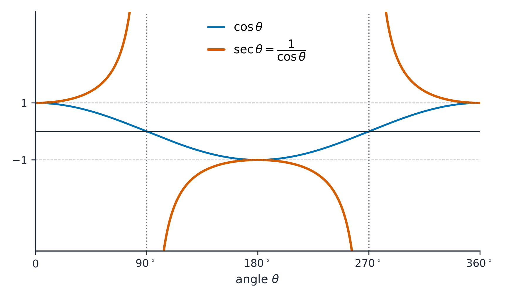
Syllabus
Learning Objective Essential Knowledge 3.11.A
Identify key characteristics of functions that involve quotients of the sine and cosine functions.- 3.11.A.1 The secant function, $f(\theta) = \sec\theta$, is the reciprocal of the cosine function, where $\cos\theta \neq 0$.
- 3.11.A.2 The cosecant function, $f(\theta) = \csc\theta$, is the reciprocal of the sine function, where $\sin\theta \neq 0$.
- 3.11.A.3 The graphs of the secant and cosecant functions have vertical asymptotes where cosine and sine are zero, respectively, and have a range of $(-\infty, -1] \cup [1, \infty)$.
- 3.11.A.4 The cotangent function, $f(\theta) = \cot\theta$, is the reciprocal of the tangent function, where $\tan\theta \neq 0$. Equivalently, $\cot\theta = \dfrac{\cos\theta}{\sin\theta}$, where $\sin\theta \neq 0$.
- 3.11.A.5 The graph of the cotangent function has vertical asymptotes for domain values where $\tan\theta = 0$ and is decreasing between consecutive asymptotes.
Source: College Board AP Course and Exam Description
These are the reciprocals 倒数 of the main three:
$$\sec\theta=\frac{1}{\cos\theta},\qquad \csc\theta=\frac{1}{\sin\theta},\qquad \cot\theta=\frac{1}{\tan\theta}.$$Secant and cosecant have vertical asymptotes where cosine and sine are zero; cotangent has them where tangent is zero (where sine is zero).sec is the reciprocal of cos, with asymptotes where cos is zero Vocabulary TrainEnglish reciprocals/rɪˈsɪprəklz/ 3.12
Equivalent Representations of Trigonometric Functions
Syllabus
Learning Objective Essential Knowledge 3.12.A
Rewrite trigonometric expressions in equivalent forms with the Pythagorean identity.- 3.12.A.1 The Pythagorean Theorem can be applied to right triangles with points on the unit circle at coordinates $(\cos\theta, \sin\theta)$, resulting in the Pythagorean identity: $\sin^2\theta + \cos^2\theta = 1$.
- 3.12.A.2 The Pythagorean identity can be algebraically manipulated into other forms involving trigonometric functions, such as $\tan^2\theta = \sec^2\theta - 1$, and can be used to establish other trigonometric relationships, such as $\arcsin x = \arccos\left(\sqrt{1 - x^2}\right)$, with appropriate domain restrictions.
3.12.B
Rewrite trigonometric expressions in equivalent forms with sine and cosine sum identities.- 3.12.B.1 The sum identity for sine is $\sin(\alpha + \beta) = \sin\alpha\cos\beta + \cos\alpha\sin\beta$.
- 3.12.B.2 The sum identity for cosine is $\cos(\alpha + \beta) = \cos\alpha\cos\beta - \sin\alpha\sin\beta$.
- 3.12.B.3 The sum identities for sine and cosine can also be used as difference and double-angle identities.
- 3.12.B.4 Properties of trigonometric functions, known trigonometric identities, and other algebraic properties can be used to verify additional trigonometric identities.
3.12.C
Solve equations using equivalent analytic representations of trigonometric functions.- 3.12.C.1 A specific equivalent form involving trigonometric expressions can make information more accessible.
- 3.12.C.2 Equivalent trigonometric forms may be useful in solving trigonometric equations and inequalities.
Source: College Board AP Course and Exam Description
The Pythagorean identity 毕达哥拉斯恒等式 comes from $x^2+y^2=1$ on the unit circle:
$$\sin^2\theta+\cos^2\theta=1,$$which rearranges into forms with $\sec$ and $\tan$. The sum identities 和角公式:$$\sin(\alpha+\beta)=\sin\alpha\cos\beta+\cos\alpha\sin\beta,\qquad \cos(\alpha+\beta)=\cos\alpha\cos\beta-\sin\alpha\sin\beta,$$also give the difference and double-angle 二倍角 identities (set $\beta=\alpha$).Vocabulary TrainEnglish Pythagorean identity/ˈpaɪθəɡɔːrɪən aɪˈdentɪti/ sum identities/sʌm aɪˈdentɪtiz/ double-angle/ˈdʌbl ˈæŋɡl/ 3.13
Trigonometry and Polar Coordinates
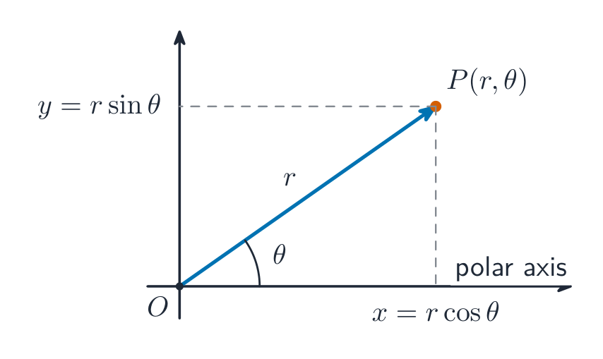
Syllabus
Learning Objective Essential Knowledge 3.13.A
Determine the location of a point in the plane using both rectangular and polar coordinates.- 3.13.A.1 The polar coordinate system is based on a grid of circles centered at the origin and on lines through the origin. Polar coordinates are defined as an ordered pair, $(r, \theta)$, such that $|r|$ represents the radius of the circle on which the point lies, and $\theta$ represents the measure of an angle in standard position whose terminal ray includes the point. In the polar coordinate system, the same point can be represented many ways.
- 3.13.A.2 The coordinates of a point in the polar coordinate system, $(r, \theta)$, can be converted to coordinates in the rectangular coordinate system, $(x, y)$, using $x = r\cos\theta$ and $y = r\sin\theta$.
- 3.13.A.3 The coordinates of a point in the rectangular coordinate system, $(x, y)$, can be converted to coordinates in the polar coordinate system, $(r, \theta)$, using $r = \sqrt{x^2 + y^2}$ and $\theta = \arctan\left(\dfrac{y}{x}\right)$ for $x > 0$ or $\theta = \arctan\left(\dfrac{y}{x}\right) + \pi$ for $x < 0$.
- 3.13.A.4 A complex number can be understood as a point in the complex plane and can be determined by its corresponding rectangular or polar coordinates. When the complex number has the rectangular coordinates $(a, b)$, it can be expressed as $a + bi$. When the complex number has polar coordinates $(r, \theta)$, it can be expressed as $(r\cos\theta) + i(r\sin\theta)$.
Source: College Board AP Course and Exam Description
Polar coordinates 极坐标 locate a point by $(r,\theta)$ – distance $r$ from the origin at angle $\theta$. Convert with
$$x=r\cos\theta,\quad y=r\sin\theta,\qquad r=\sqrt{x^2+y^2},\quad \tan\theta=\frac{y}{x}.$$A complex number 复数 is the point $(x,y)=x+yi$ and can likewise be written with $r$ and $\theta$.Polar coordinates give a point by its distance r and angle theta Vocabulary TrainEnglish Polar coordinates/ˈpəʊlə kəʊˈɔːdɪnəts/ complex number/ˈkɒmpleks ˈnʌmbə/ 3.14
Polar Function Graphs
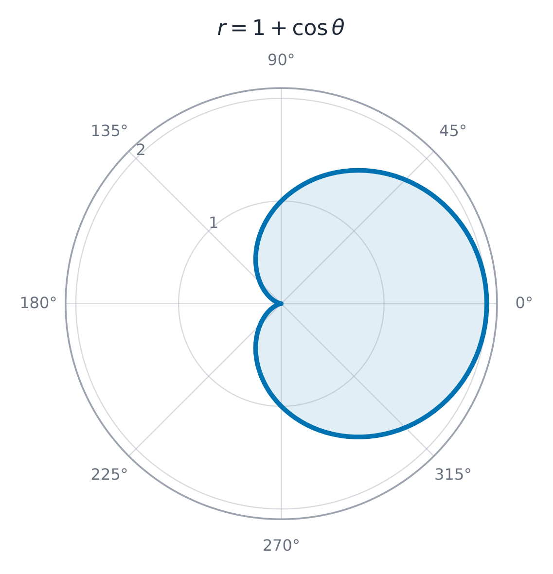
Syllabus
Learning Objective Essential Knowledge 3.14.A
Construct graphs of polar functions.- 3.14.A.1 The graph of the function $r = f(\theta)$ in polar coordinates consists of input-output pairs of values where the input values are angle measures and the output values are radii.
- 3.14.A.2 The domain of the polar function $r = f(\theta)$, given graphically, can be restricted to a desired portion of the function by selecting endpoints corresponding to the desired angle and radius.
- 3.14.A.3 When graphing polar functions in the form of $r = f(\theta)$, changes in input values correspond to changes in angle measure from the positive $x$-axis, and changes in output values correspond to changes in distance from the origin.
Source: College Board AP Course and Exam Description
Tracing a polar curve The graph of $r=f(\theta)$ is all points $(r,\theta)$ as $\theta$ sweeps around. Restricting the domain of $\theta$ draws only part of the curve. As $\theta$ increases, $r$ grows or shrinks, tracing spirals, circles, roses, and limaçons.
A cardioid r = 1 + cos theta, sketched directly in polar form ExplorePlot a curve in polar coordinates
In polar form a point is a distance $r$ at angle $\theta$. Letting $r$ depend on $\theta$ traces shapes a rule in $x,y$ can't — like this cardioid.
3.15
Rates of Change in Polar Functions
Syllabus
Learning Objective Essential Knowledge 3.15.A
Describe characteristics of the graph of a polar function.- 3.15.A.1 If a polar function, $r = f(\theta)$, is positive and increasing or negative and decreasing, then the distance between $f(\theta)$ and the origin is increasing.
- 3.15.A.2 If a polar function, $r = f(\theta)$, is positive and decreasing or negative and increasing, then the distance between $f(\theta)$ and the origin is decreasing.
- 3.15.A.3 For a polar function, $r = f(\theta)$, if the function changes from increasing to decreasing or decreasing to increasing on an interval, then the function has a relative extremum on the interval corresponding to a point relatively closest to or farthest from the origin.
- 3.15.A.4 The average rate of change of $r$ with respect to $\theta$ over an interval of $\theta$ is the ratio of the change in the radius values to the change in $\theta$ over an interval of $\theta$. Graphically, the average rate of change indicates the rate at which the radius is changing per radian.
- 3.15.A.5 The average rate of change of $r$ with respect to $\theta$ over an interval of $\theta$ can be used to estimate values of the function within the interval.
Source: College Board AP Course and Exam Description
As $\theta$ increases, the distance from the origin $r$ changes:
- $r$ positive and increasing (or negative and decreasing) $\Rightarrow$ moving away from the origin;
- $r$ positive and decreasing (or negative and increasing) $\Rightarrow$ moving toward the origin.
Where $r$ switches between increasing and decreasing, the distance reaches a relative extreme. The average rate of change of $r$ with respect to $\theta$, $\dfrac{\Delta r}{\Delta \theta}$, estimates how fast the curve moves in or out over an interval.
3.15
Exam tips
- Use radians and the unit circle: $\cos\theta$ and $\sin\theta$ are the coordinates, always between $-1$ and $1$.
- For a sinusoid $a\sin(b(\theta+c))+d$: $|a|$ is the amplitude, $\tfrac{2\pi}{|b|}$ the period, $d$ the midline, and the phase shift is $-c$ (a $+c$ shifts left).
- Model periodic data by reading period, amplitude, and midline from the max and min.
- Inverse trig functions need a restricted domain and return an angle; trig equations have infinitely many solutions (add the period).
- Convert polar↔rectangular with $x=r\cos\theta$, $y=r\sin\theta$.
-
4
Functions Involving Parameters, Vectors, and Matrices
Watch lesson4.1
Parametric Functions

Syllabus
Learning Objective Essential Knowledge 4.1.A
Construct a graph or table of values for a parametric function represented analytically.- 4.1.A.1 A parametric function in $\mathbb{R}^2$, the set of all ordered pairs of two real numbers, consists of a set of two parametric equations in which two dependent variables, $x$ and $y$, are dependent on a single independent variable, $t$, called the parameter.
- 4.1.A.2 Because variables $x$ and $y$ are dependent on the independent variable, $t$, the coordinates $(x_i,\, y_i)$ at time $t_i$ can be written as functions of $t$ and can be expressed as the single parametric function $f(t) = (x(t),\, y(t))$, where in this case $x$ and $y$ are names of two functions.
- 4.1.A.3 A numerical table of values can be generated for the parametric function $f(t) = (x(t),\, y(t))$ by evaluating $x_i$ and $y_i$ at several values of $t_i$ within the domain.
- 4.1.A.4 A graph of a parametric function can be sketched by connecting several points from the numerical table of values in order of increasing value of $t$.
- 4.1.A.5 The domain of the parametric function $f$ is often restricted, which results in start and end points on the graph of $f$.
Source: College Board AP Course and Exam Description
A roller coaster: vectors and parametric motion describe path and velocity together Unit 4 is part of the course but is not assessed on the AP Precalculus Exam (which covers only Units 1–3); it builds tools used in later courses.
A parametric function 参数函数 describes a curve by giving both coordinates as functions of a third variable, the parameter 参数 $t$: $\big(x(t),\,y(t)\big)$. As $t$ runs through its domain, the point traces a path – and, unlike $y=f(x)$, the path may loop or cross itself.
Vocabulary TrainEnglish parametric function/ˌpærəˈmetrɪk ˈfʌŋkʃn/ parameter/pəˈræmɪtə/ 4.2
Parametric Functions and Planar Motion
Syllabus
Learning Objective Essential Knowledge 4.2.A
Identify key characteristics of a parametric planar motion function that are related to position.- 4.2.A.1 A parametric function given by $f(t) = (x(t),\, y(t))$ can be used to model particle motion in the plane. The graph of this function indicates the position of a particle at time $t$.
- 4.2.A.2 The horizontal and vertical extrema of a particle's motion can be determined by identifying the maximum and minimum values of the functions $x(t)$ and $y(t)$, respectively.
- 4.2.A.3 The real zeros of the function $x(t)$ correspond to $y$-intercepts, and the real zeros of $y(t)$ correspond to $x$-intercepts.
Source: College Board AP Course and Exam Description
Reading $t$ as time, a parametric function models motion in the plane. $x(t)$ and $y(t)$ give the horizontal and vertical position; the point's direction of travel is the order in which the curve is drawn as $t$ increases (mark it with arrows).
4.3
Parametric Functions and Rates of Change
Syllabus
Learning Objective Essential Knowledge 4.3.A
Identify key characteristics of a parametric planar motion function that are related to direction and rate of change.- 4.3.A.1 As the parameter increases, the direction of planar motion of a particle can be analyzed in terms of $x$ and $y$ independently. If $x(t)$ is increasing or decreasing, the direction of motion is to the right or left, respectively. If $y(t)$ is increasing or decreasing, the direction of motion is up or down, respectively.
- 4.3.A.2 At any given point in the plane, the direction of planar motion may be different for different values of $t$.
- 4.3.A.3 The same curve in the plane can be parametrized in different ways and can be traversed in different directions with different parametric functions.
- 4.3.A.4 Over a given interval $[t_1,\, t_2]$ within the domain, the average rate of change can be computed for $x(t)$ and $y(t)$ independently. The ratio of the average rate of change of $y$ to the average rate of change of $x$ gives the slope of the graph between the points on the curve corresponding to $t_1$ and $t_2$, so long as the average rate of change of $x(t) \neq 0$.
Source: College Board AP Course and Exam Description
Over an interval of $t$, the average rate of change of $x$ is $\dfrac{\Delta x}{\Delta t}$ and of $y$ is $\dfrac{\Delta y}{\Delta t}$. Their signs tell you which way the point moves (right/left, up/down); together they describe the motion's speed and direction along the path.
4.4
Parametrically Defined Circles and Lines
Syllabus
Learning Objective Essential Knowledge 4.4.A
Express motion around a circle or along a line segment parametrically.- 4.4.A.1 A complete counterclockwise revolution around the unit circle that starts and ends at $(1,\, 0)$ and is centered at the origin can be modeled by $(x(t),\, y(t)) = (\cos t,\, \sin t)$ with domain $0 \leq t \leq 2\pi$.
- 4.4.A.2 Transformations of the parametric function $(x(t),\, y(t)) = (\cos t,\, \sin t)$ can model any circular path traversed in the plane.
- 4.4.A.3 A linear path along the line segment from the point $(x_1,\, y_1)$ to the point $(x_2,\, y_2)$ can be parametrized many ways, including using an initial position $(x_1,\, y_1)$ and rates of change for $x$ with respect to $t$ and $y$ with respect to $t$.
Source: College Board AP Course and Exam Description
A circle of radius $R$ centered at $(h,k)$ is $x=h+R\cos t,\ y=k+R\sin t$. A line through $(x_0,y_0)$ with direction $(a,b)$ is $x=x_0+at,\ y=y_0+bt$. Adjusting the coefficients changes the start point, speed, and direction of tracing.
4.5
Implicitly Defined Functions
Syllabus
Learning Objective Essential Knowledge 4.5.A
Construct a graph of an equation involving two variables.- 4.5.A.1 An equation involving two variables can implicitly describe one or more functions.
- 4.5.A.2 An equation involving two variables can be graphed by finding solutions to the equation.
- 4.5.A.3 Solving for one of the variables in an equation involving two variables can define a function whose graph is part or all of the graph of the equation.
4.5.B
Determine how the two quantities related in an implicitly defined function vary together.- 4.5.B.1 For ordered pairs on the graph of an implicitly defined function that are close together, if the ratio of the change in the two variables is positive, then the two variables simultaneously increase or both decrease; conversely, if the ratio is negative, then as one variable increases, the other decreases.
- 4.5.B.2 The rate of change of $x$ with respect to $y$ or of $y$ with respect to $x$ can be zero, indicating vertical or horizontal intervals, respectively.
Source: College Board AP Course and Exam Description
An implicit 隐式 equation relates $x$ and $y$ without solving for either, such as $x^2+y^2=25$. Its graph may fail the vertical-line test (not a function), so it is often split into pieces or described parametrically.
Vocabulary TrainEnglish implicit/ɪmˈplɪsɪt/ 4.6
Conic Sections
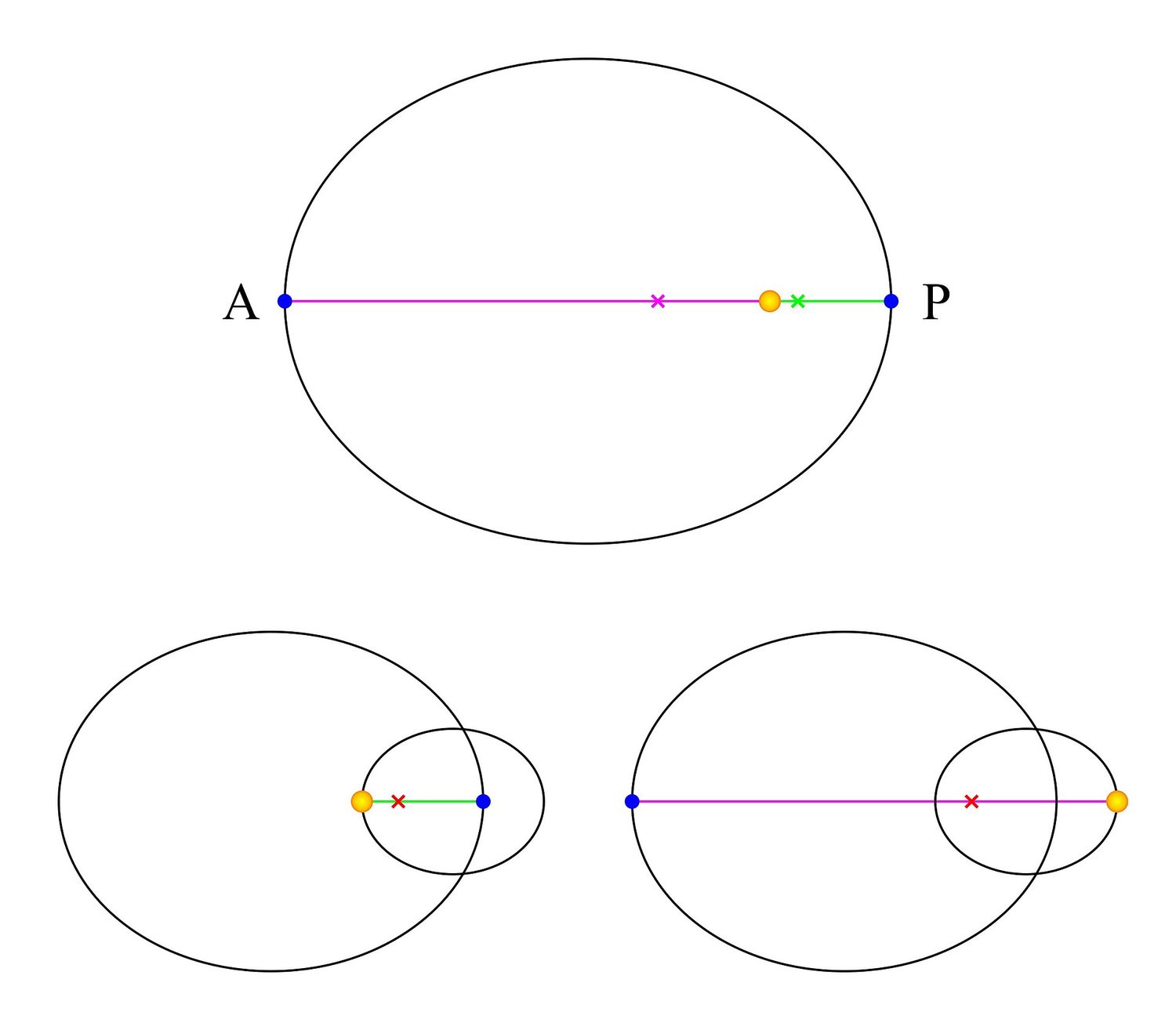
Syllabus
Learning Objective Essential Knowledge 4.6.A
Represent conic sections with horizontal or vertical symmetry analytically.- 4.6.A.1 A parabola with vertex $(h,\, k)$ can, if $a \neq 0$, be represented analytically as $x - h = a(y - k)^2$ if it opens left or right, or as $y - k = a(x - h)^2$ if it opens up or down.
- 4.6.A.2 An ellipse centered at $(h,\, k)$ with horizontal radius $a$ and vertical radius $b$ can be represented analytically as $\dfrac{(x - h)^2}{a^2} + \dfrac{(y - k)^2}{b^2} = 1$. A circle is a special case of an ellipse where $a = b$.
- 4.6.A.3 A hyperbola centered at $(h,\, k)$ with vertical and horizonal lines of symmetry can be represented algebraically as $\dfrac{(x - h)^2}{a^2} - \dfrac{(y - k)^2}{b^2} = 1$ for a hyperbola opening left and right, or as $\dfrac{(y - k)^2}{b^2} - \dfrac{(x - h)^2}{a^2} = 1$ for a hyperbola opening up and down. The asymptotes are $y - k = \pm \dfrac{b}{a}(x - h)$.
Source: College Board AP Course and Exam Description
Conic sections: one cone, four curves Conic sections 圆锥曲线 – circles, ellipses, parabolas, and hyperbolas – are the curves from slicing a cone, each given by a quadratic equation in $x$ and $y$. Their standard forms reveal centers, vertices, axes, and asymptotes.
Elliptical orbits: conic sections describe closed paths with two foci — a key parametric model Vocabulary TrainEnglish Conic sections/ˈkɒnɪk ˈsekʃnz/ 4.7
Parametrizing Implicit Curves
Syllabus
Learning Objective Essential Knowledge 4.7.A
Represent a curve in the plane parametrically.- 4.7.A.1 A parametrization $(x(t),\, y(t))$ for an implicitly defined function will, when $x(t)$ and $y(t)$ are substituted for $x$ and $y$, respectively, satisfy the corresponding equation for every value of $t$ in the domain.
- 4.7.A.2 If $f$ is a function of $x$, then $y = f(x)$ can be parametrized as $(x(t),\, y(t)) = (t, f(t))$. If $f$ is invertible, its inverse can be parametrized as $(x(t),\, y(t)) = (f(t),\, t)$ for an appropriate interval of $t$.
4.7.B
Represent conic sections parametrically.- 4.7.B.1 A parabola can be parametrized in the same way that any equation that can be solved for $x$ or $y$ can be parametrized. Equations that can be solved for $x$ can be parametrized as $(x(t),\, y(t)) = (f(t),\, t)$ by solving for $x$ and replacing $y$ with $t$. Equations that can be solved for $y$ can be parametrized as $(x(t),\, y(t)) = (t, f(t))$ by solving for $y$ and replacing $x$ with $t$.
- 4.7.B.2 An ellipse can be parametrized using the trigonometric functions $x(t) = h + a\cos t$ and $y(t) = k + b\sin t$ for $0 \leq t \leq 2\pi$.
- 4.7.B.3 A hyperbola can be parametrized using trigonometric functions. For a hyperbola that opens left and right, the functions are $x(t) = h + a\sec t$ and $y(t) = k + b\tan t$ for $0 \leq t \leq 2\pi$. For a hyperbola that opens up and down, the functions are $x(t) = h + a\tan t$ and $y(t) = k + b\sec t$ for $0 \leq t \leq 2\pi$.
Source: College Board AP Course and Exam Description
Many implicit curves can be parametrized – rewritten as $\big(x(t),y(t)\big)$ – which makes them easier to graph and to treat as motion. The circle above is the basic example; ellipses use $x=h+A\cos t,\ y=k+B\sin t$.
4.8
Vectors
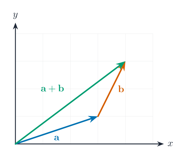
Syllabus
Learning Objective Essential Knowledge 4.8.A
Identify characteristics of a vector.- 4.8.A.1 A vector is a directed line segment. When a vector is placed in the plane, the point at the beginning of the line segment is called the tail, and the point at the end of the line segment is called the head. The length of the line segment is the magnitude of the vector.
- 4.8.A.2 A vector $\overrightarrow{P_1 P_2}$ with two components can be plotted in the $xy$-plane from $P_1 = (x_1, y_1)$ to $P_2 = (x_2, y_2)$. The vector is identified by $a$ and $b$, where $a = x_2 - x_1$ and $b = y_2 - y_1$. The vector can be expressed as $\langle a,\, b \rangle$. A zero vector $\langle 0,\, 0 \rangle$ is the trivial case when $P_1 = P_2$.
- 4.8.A.3 The direction of the vector is parallel to the line segment from the origin to the point with coordinates $(a,\, b)$. The magnitude of the vector is the square root of the sum of the squares of the components.
- 4.8.A.4 For a vector represented geometrically in the plane, the components of the vector can be found using trigonometry.
4.8.B
Determine sums and products involving vectors.- 4.8.B.1 The multiplication of a constant and a vector results in a new vector whose components are found by multiplying the constant by each of the components of the original vector. The new vector is parallel to the original vector.
- 4.8.B.2 The sum of two vectors in $\mathbb{R}^2$ is a new vector whose components are found by adding the corresponding components of the original vectors. The new vector can be represented graphically as a vector whose tail corresponds to the tail of the first vector and whose head corresponds to the head of the second vector when the second vector's tail is located at the first vector's head.
- 4.8.B.3 The dot product of two vectors is the sum of the products of their corresponding components. That is, $\langle a_1,\, b_1 \rangle \cdot \langle a_2,\, b_2 \rangle = a_1 a_2 + b_1 b_2$.
4.8.C
Determine a unit vector for a given vector.- 4.8.C.1 A unit vector is a vector of magnitude $1$. A unit vector in the same direction as a given nonzero vector can be found by scalar multiplying the vector by the reciprocal of its magnitude.
- 4.8.C.2 The vector $\langle a,\, b \rangle$ can be expressed as $a\vec{i} + b\vec{j}$ in $\mathbb{R}^2$, where $\vec{i}$ and $\vec{j}$ are unit vectors in the $x$ and $y$ directions, respectively. That is, $\vec{i} = \langle 1,\, 0 \rangle$ and $\vec{j} = \langle 0,\, 1 \rangle$.
4.8.D
Determine angle measures between vectors and magnitudes of vectors involved in vector addition.- 4.8.D.1 The dot product is geometrically equivalent to the product of the magnitudes of the two vectors and the cosine of the angle between them. Therefore, if the dot product of two nonzero vectors is zero, then the vectors are perpendicular.
- 4.8.D.2 The Law of Sines and Law of Cosines can be used to determine side lengths and angle measures of triangles formed by vector addition.
Source: College Board AP Course and Exam Description
Resolving a vector into components A vector 向量 has both magnitude 大小 (length) and direction. Write it by components $\langle a,b\rangle$. Add vectors component-by-component; scale by multiplying each component; the magnitude is $\sqrt{a^2+b^2}$. Vectors model displacements, velocities, and forces.
Adding vectors by the triangle law ExploreAdd two vectors tip to tail
A vector has magnitude and direction. Adding two vectors places them tip to tail; the resultant runs from the first tail to the last tip. Drag each to see the sum.
Vocabulary TrainEnglish vector/ˈvektə/ magnitude/ˈmæɡnɪtjuːd/ 4.9
Vector-Valued Functions
Syllabus
Learning Objective Essential Knowledge 4.9.A
Represent planar motion in terms of vector-valued functions.- 4.9.A.1 The position of a particle moving in a plane that is given by the parametric function $f(t) = (x(t),\, y(t))$ may be expressed as a vector-valued function, $p(t) = x(t)\vec{i} + y(t)\vec{j}$ or $p(t) = \langle x(t),\, y(t) \rangle$. The magnitude of the position vector at time $t$ gives the distance of the particle from the origin.
- 4.9.A.2 The vector-valued function $v(t) = \langle x(t),\, y(t) \rangle$ can be used to express the velocity of a particle moving in a plane at different times, $t$. At time $t$, the sign of $x(t)$ indicates if the particle is moving right or left, and the sign of $y(t)$ indicates if the particle is moving up or down. The magnitude of the velocity vector at time $t$ gives the speed of the particle.
Source: College Board AP Course and Exam Description
A vector-valued function 向量值函数 outputs a vector for each input, e.g. $\vec{r}(t)=\langle x(t),y(t)\rangle$ – the same information as a parametric function, packaged as a moving position vector.
A vector-valued line: start at a, then slide by t lots of the direction b Vocabulary TrainEnglish vector-valued function/ˈvektə ˈvæljuːd ˈfʌŋkʃn/ 4.10
Matrices
Syllabus
Learning Objective Essential Knowledge 4.10.A
Determine the product of two matrices.- 4.10.A.1 An $n \times m$ matrix is an array consisting of $n$ rows and $m$ columns.
- 4.10.A.2 Two matrices can be multiplied if the number of columns in the first matrix equals the number of rows in the second matrix. The product of the matrices is a new matrix in which the component in the $i$th row and $j$th column is the dot product of the $i$th row of the first matrix and the $j$th column of the second matrix.
Source: College Board AP Course and Exam Description
A matrix 矩阵 is a rectangular array of numbers. Add matrices of the same size entry-by-entry; multiply a matrix by a compatible one by combining rows with columns. Matrices store and transform data compactly.
Vocabulary TrainEnglish matrix/ˈmeɪtrɪks/ 4.11
The Inverse and Determinant of a Matrix
Syllabus
Learning Objective Essential Knowledge 4.11.A
Determine the inverse of a $2 \times 2$ matrix.- 4.11.A.1 The identity matrix, $I$, is a square matrix consisting of $1$s on the diagonal from the top left to bottom right and $0$s everywhere else.
- 4.11.A.2 Multiplying a square matrix by its corresponding identity matrix results in the original square matrix.
- 4.11.A.3 The product of a square matrix and its inverse, when it exists, is the identity matrix of the same size.
- 4.11.A.4 The inverse of a $2 \times 2$ matrix, when it exists, can be calculated with or without technology.
4.11.B
Apply the value of the determinant to invertibility and vectors.- 4.11.B.1 The determinant of the matrix $A = \begin{bmatrix} a & b \\ c & d \end{bmatrix}$ is $ad - bc$. The determinant can be calculated with or without technology and is denoted $\det(A)$.
- 4.11.B.2 If a $2 \times 2$ matrix consists of two column or row vectors from $\mathbb{R}^2$, then the nonzero absolute value of the determinant of the matrix is the area of the parallelogram spanned by the vectors represented in the columns or rows of the matrix. If the determinant equals $0$, then the vectors are parallel.
- 4.11.B.3 The square matrix $A$ has an inverse if and only if $\det(A) \neq 0$.
Source: College Board AP Course and Exam Description
The determinant 行列式 of a $2\times 2$ matrix $\begin{bmatrix} a & b \\ c & d\end{bmatrix}$ is $ad-bc$. A matrix has an inverse 逆矩阵 exactly when its determinant is nonzero; the inverse undoes the matrix, and it solves matrix equations (like a reciprocal for numbers).
Worked example. For $A=\begin{bmatrix}3 & 1\\ 2 & 4\end{bmatrix}$, the determinant is $ad-bc=(3)(4)-(1)(2)=10$. Since it is nonzero, $A$ is invertible, and $A^{-1}=\dfrac{1}{10}\begin{bmatrix}4 & -1\\ -2 & 3\end{bmatrix}$ (swap the diagonal, negate the off-diagonal, divide by the determinant).
Vocabulary TrainEnglish determinant/dɪˈtɜːmɪnənt/ inverse/ɪnˈvɜːs/ 4.12
Linear Transformations and Matrices
Syllabus
Learning Objective Essential Knowledge 4.12.A
Determine the output vectors of a linear transformation using a $2 \times 2$ matrix.- 4.12.A.1 A linear transformation is a function that maps an input vector to an output vector such that each component of the output vector is the sum of constant multiples of the input vector components.
- 4.12.A.2 A linear transformation will map the zero vector to the zero vector.
- 4.12.A.3 A single vector in $\mathbb{R}^2$ can be expressed as a $2 \times 1$ matrix. A set of $n$ vectors in $\mathbb{R}^2$ can be expressed as a $2 \times n$ matrix.
- 4.12.A.4 For a linear transformation, $L$, from $\mathbb{R}^2$ to $\mathbb{R}^2$, there is a unique $2 \times 2$ matrix, $A$, such that $L(\vec{v}) = A\vec{v}$ for vectors in $\mathbb{R}^2$. Conversely, for a given $2 \times 2$ matrix, $A$, the function $L(\vec{v}) = A\vec{v}$ is a linear transformation from $\mathbb{R}^2$ to $\mathbb{R}^2$.
- 4.12.A.5 Multiplication of a $2 \times 2$ transformation matrix, $A$, and a $2 \times n$ matrix of $n$ input vectors gives a $2 \times n$ matrix of the $n$ output vectors for the linear transformation $L(\vec{v}) = A\vec{v}$.
Source: College Board AP Course and Exam Description
A matrix transforms the plane A $2\times 2$ matrix acts as a linear transformation 线性变换 of the plane – rotating, reflecting, stretching, or shearing points – by multiplying each position vector. The determinant measures how the transformation scales area (and its sign tells whether orientation flips).
Worked example. The matrix $\begin{bmatrix}2 & 0\\ 0 & 3\end{bmatrix}$ stretches the plane by $2$ horizontally and $3$ vertically, sending the vector $\begin{bmatrix}1\\1\end{bmatrix}$ to $\begin{bmatrix}2\\3\end{bmatrix}$. Its determinant $2\times3=6$ means every area is multiplied by $6$, so the unit square becomes a $2\times3$ rectangle.
A 2x2 matrix maps the unit square to a parallelogram; the determinant is the area scale ExploreTransform the plane with a matrix
A $2\times2$ matrix maps every point to a new one, so it stretches, rotates or shears the whole grid. Change the entries and watch the unit square transform.
Vocabulary TrainEnglish linear transformation/ˈlɪnɪə trænsfɔːˈmeɪʃn/ 4.13
Matrices as Functions
Syllabus
Learning Objective Essential Knowledge 4.13.A
Determine the association between a linear transformation and a matrix.- 4.13.A.1 The linear transformation mapping $\langle x,\, y \rangle$ to $\langle a_{11} x + a_{12} y,\, a_{21} x + a_{22} y \rangle$ is associated with the matrix $\begin{bmatrix} a_{11} & a_{12} \\ a_{21} & a_{22} \end{bmatrix}$.
- 4.13.A.2 The mapping of the unit vectors in a linear transformation provides valuable information for determining the associated matrix.
- 4.13.A.3 The matrix $\begin{bmatrix} \cos\theta & -\sin\theta \\ \sin\theta & \cos\theta \end{bmatrix}$ is associated with a linear transformation of vectors that rotates every vector an angle $\theta$ counterclockwise about the origin.
- 4.13.A.4 The absolute value of the determinant of a $2 \times 2$ transformation matrix gives the magnitude of the dilation of regions in $\mathbb{R}^2$ under the transformation.
4.13.B
Determine the composition of two linear transformations.- 4.13.B.1 The composition of two linear transformations is a linear transformation.
- 4.13.B.2 The matrix associated with the composition of two linear transformations is the product of the matrices associated with each linear transformation.
4.13.C
Determine the inverse of a linear transformation.- 4.13.C.1 Two linear transformations are inverses if their composition maps any vector to itself.
- 4.13.C.2 If a linear transformation, $L$, is given by $L(\vec{v}) = A\vec{v}$, then its inverse transformation is given by $L^{-1}(\vec{v}) = A^{-1}\vec{v}$, where $A^{-1}$ is the inverse of the matrix $A$.
Source: College Board AP Course and Exam Description
Because a matrix maps input vectors to output vectors, it is a function on the plane. Composing transformations corresponds to multiplying their matrices, and the inverse matrix reverses the mapping.
4.14
Matrices Modeling Contexts
Syllabus
Learning Objective Essential Knowledge 4.14.A
Construct a model of a scenario involving transitions between two states using matrices.- 4.14.A.1 A contextual scenario can indicate the rate of transitions between states as percent changes. A matrix can be constructed based on these rates to model how states change over discrete intervals.
4.14.B
Apply matrix models to predict future and past states for $n$ transition steps.- 4.14.B.1 The product of a matrix that models transitions between states and a corresponding state vector can predict future states.
- 4.14.B.2 Repeated multiplication of a matrix that models the transitions between states and corresponding resultant state vectors can predict the steady state, a distribution between states that does not change from one step to the next.
- 4.14.B.3 The product of the inverse of a matrix that models transitions between states and a corresponding state vector can predict past states.
Source: College Board AP Course and Exam Description
Matrices model systems that step forward in stages – for example, populations moving between states each year. Repeated multiplication by a transition matrix advances the model one step at a time, so matrix powers predict long-run behavior.
4.14
Exam tips
- A parametric function gives $x(t)$ and $y(t)$ separately — track the direction of motion as $t$ increases.
- A vector has magnitude and direction; add component-by-component and find magnitude with $\sqrt{a^2+b^2}$.
- The determinant of a $2\times2$ matrix is $ad-bc$ (mind the minus sign); it scales area under the transformation.
- A $2\times2$ matrix transforms the plane (rotate, reflect, stretch); an inverse exists only when the determinant is non-zero.
- Note this unit is not tested on the AP Precalculus Exam (Units 1–3 only), but it underpins later courses.