Comparing algorithms and ADTs in algorithms · 比较算法与算法中的 ADT
| English | 中文 | Pinyin · 拼音 |
|---|---|---|
| Big-O/bɪɡ əʊ/ | 大O表示法 | dà O biǎo shì fǎ |
| time complexity/taɪm kəmˈpleksɪti/ | 时间复杂度 | shí jiān fù zá dù |
| space complexity/speɪs kəmˈpleksɪti/ | 空间复杂度 | kōng jiān fù zá dù |
| depth-first/depθ fɜːst/ | 深度优先 | shēn dù yōu xiān |
| breadth-first/bredθ fɜːst/ | 广度优先 | guǎng dù yōu xiān |
| binary tree/ˈbaɪnəri triː/ | 二叉树 | èr chā shù |
The algorithm that would outlive the universe
- A salesman must visit 25 cities and return home by the shortest route. Try every order and there are about $10^{23}$ of them. A machine checking a billion a second would take three million years.
- Add one more city and the work multiplies by 25. That is not a computer that needs to be faster; it is an approach that can never work, at any speed, on any hardware.
- Knowing that before you write the program is what complexity analysis is for. It is the difference between choosing an algorithm and discovering, months later, that yours does not scale.
- This lesson is Big-O 大O表示法 for time and space, and how ADTs shape the algorithms built on them.
会比宇宙活得更久的算法
- 一位推销员必须访问 25 座城市并按最短路线回家。把每种顺序都试一遍,大约有 $10^{23}$ 种。一台每秒检查十亿种的机器要花三百万年。
- 再加一座城市,工作量乘以 25。这不是一台需要更快的计算机;这是一种在任何速度、任何硬件上都永远行不通的方法。
- 在写程序之前就知道这一点,正是复杂度分析的用途。它是"选择一个算法"和"几个月后发现你的算法扩展不了"之间的差别。
- 这一课讲时间和空间的大O表示法(Big-O),以及抽象数据类型怎样塑造建立在它们之上的算法。
Time complexity
- Time complexity 时间复杂度 describes how the running time grows with the input size $n$. It is written in Big-O notation, which keeps only the dominant term and drops constants.
- $O(1)$ constant, the time does not depend on $n$ at all. $O(\log n)$ logarithmic, as in binary search. $O(n)$ linear, as in linear search. $O(n \log n)$, the good sorts. $O(n^2)$ quadratic, as in bubble and insertion sort.
- The reason constants are dropped: they are swamped. An $O(n^2)$ algorithm might beat an $O(n \log n)$ one for $n = 10$, but at $n = 10{,}000$ nothing about the constants can save it.
The curves cross once, and after that the order decides everything
时间复杂度
- 时间复杂度(time complexity)描述运行时间怎样随输入规模 $n$ 增长。它用大O表示法书写,只保留主导项、丢掉常数。
- $O(1)$ 常数,时间根本不依赖 $n$。$O(\log n)$ 对数,如二分查找。$O(n)$ 线性,如线性查找。$O(n \log n)$,那些好的排序。$O(n^2)$ 平方,如冒泡和插入排序。
- 丢掉常数的理由是:它们会被淹没。一个 $O(n^2)$ 的算法在 $n = 10$ 时可能胜过 $O(n \log n)$ 的,但在 $n = 10{,}000$ 时,常数救不了它。
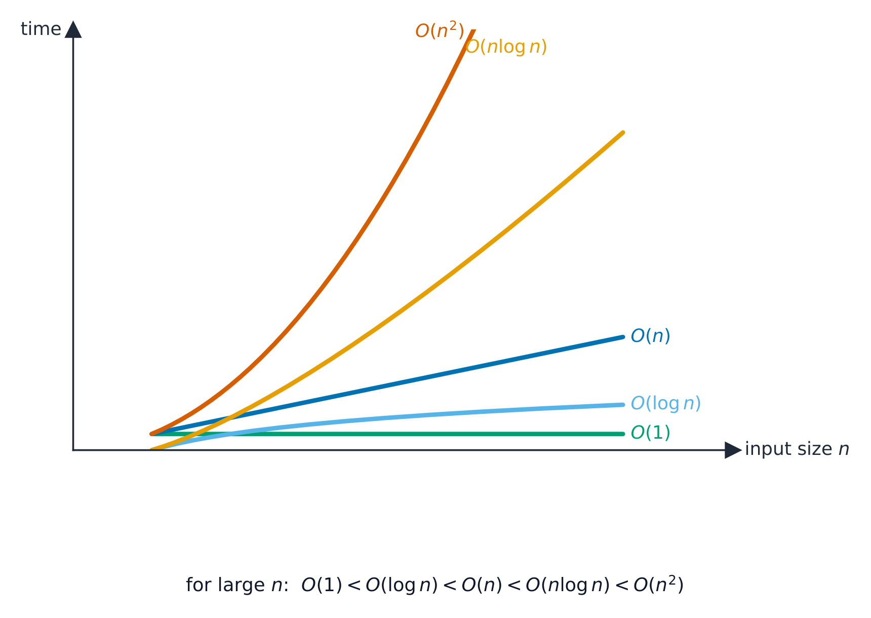
曲线只交叉一次,此后一切都由阶决定
How running time grows with n · 运行时间如何随 n 增长
Slide n upward and compare the curves: O(1) and O(log n) stay almost flat, O(n) rises steadily, O(n²) explodes. This is why Big-O — not a stopwatch — is how we compare algorithms on large inputs. · 把 n 向上滑动并比较曲线:O(1) 和 O(log n) 几乎保持平坦,O(n) 稳步上升,O(n²) 爆炸。这就是为什么大 O——而不是一个秒表——是我们在大输入上比较算法的方式。
Which Big-O describes binary search? · 哪个大 O 描述二分搜索?
Halving the range each step is logarithmic — O(log n). · 每步把范围减半是对数的——O(log n)。
Which Big-O describes bubble sort in the worst case? · 哪个大 O 描述最坏情况下的冒泡排序?
Two nested loops over n elements give O(n²). · 在 n 个元素上的两个嵌套循环给出 O(n²)。
Match each algorithm to its time complexity. · 把每个算法与它的时间复杂度配对。
Linear search is O(n), binary search O(log n), bubble sort O(n²). · 线性搜索是 O(n),二分搜索 O(log n),冒泡排序 O(n²)。
Worked example: what doubling the input does
- An algorithm takes 4 seconds on 1,000 items. Estimate its time on 2,000 items if it is $O(n)$, then if it is $O(n^2)$.
- $O(n)$: doubling $n$ doubles the time, so about 8 seconds.
- $O(n^2)$: doubling $n$ quadruples the time, so about 16 seconds. At 10,000 items it would be 100 times the original, about 400 seconds.
- $O(\log n)$ would add only a single step, and $O(1)$ would not change at all. Reason from the order, not from a formula.
例题:输入翻倍会怎样
- 一个算法处理 1000 项要 4 秒。若它是 $O(n)$,估计处理 2000 项要多久;若它是 $O(n^2)$ 呢?
- $O(n)$:$n$ 翻倍时间翻倍,所以约 8 秒。
- $O(n^2)$:$n$ 翻倍时间变为四倍,所以约 16 秒。到 10,000 项时会是原来的 100 倍,约 400 秒。
- $O(\log n)$ 只会多一步,而 $O(1)$ 根本不变。从阶来推理,不要套公式。
An O(n squared) algorithm takes 4 seconds on 1,000 items. Roughly how many seconds will it take on 2,000? · 一个 O(n 平方) 的算法处理 1000 项要 4 秒。处理 2000 项大约要几秒?
Doubling n quadruples an O(n squared) time. The same doubling would take an O(n) algorithm from 4 seconds to 8. · n 翻倍会让 O(n 平方) 的时间变四倍。同样的翻倍会让 O(n) 的算法从 4 秒变成 8 秒。
Space complexity
- Space complexity 空间复杂度 is the extra memory an algorithm needs, beyond the input itself.
- Bubble and insertion sort use $O(1)$ extra memory: they work in place, needing only a couple of variables. Merge sort uses $O(n)$, since it builds a second array.
- Recursion uses stack memory proportional to its depth, because every unfinished call keeps its own frame.
- There is often a time and memory trade-off: storing results to avoid recomputing them, as memoisation does, buys speed with space.
空间复杂度
- 空间复杂度(space complexity)是算法在输入本身之外所需的额外内存。
- 冒泡和插入排序用 $O(1)$ 的额外内存:它们原地工作,只需要几个变量。归并排序用 $O(n)$,因为它要建第二个数组。
- 递归占用的栈内存与它的深度成正比,因为每个未完成的调用都保留自己的栈帧。
- 常常存在时间与内存的取舍:像记忆化那样把结果存起来以免重算,就是用空间换速度。
What else decides the choice
- Big-O is about growth, not absolute speed. For a small $n$, a simple $O(n^2)$ algorithm can beat a complicated $O(n \log n)$ one, and it is easier to write correctly.
- Stability matters when a list is already ordered by another field. Simplicity matters because a simple algorithm has fewer places to hide a bug.
- The honest answer to "which algorithm" often names the order and the conditions: this one, because $n$ is large and the data arrives unsorted.
还有什么决定选择
- 大O说的是增长,不是绝对速度。对小的 $n$,一个简单的 $O(n^2)$ 算法可能胜过一个复杂的 $O(n \log n)$ 算法,而且更容易写对。
- 当列表已按另一个字段排过序时,稳定性很要紧。简单性也要紧,因为简单的算法能藏 bug 的地方更少。
- "选哪个算法"的诚实答案往往同时说出阶和条件:选这个,因为 $n$ 很大而且数据到达时无序。
An "in place" sort: · 一个“原地”排序:
In-place algorithms (like bubble and insertion sort) sort within the original array, using constant extra space. · 原地算法(像冒泡和插入排序)在原始数组内排序,用常数的额外空间。
Why is bubble sort's space complexity O(1) even though it sorts an array of n items? · 冒泡排序明明在给 n 个项的数组排序,为什么它的空间复杂度是 O(1)?
It sorts in place. Merge sort is O(n) because it builds a second array, and recursion costs memory proportional to its depth. · 它原地排序。归并排序是 O(n),因为它要建第二个数组;递归的内存代价与它的深度成正比。
ADTs inside algorithms
- The abstract data types from topic 10 are the machinery algorithms are built from, and choosing one shapes the algorithm.
- A stack gives depth-first 深度优先 search: push the neighbours, take the most recent, and the search plunges down one path before backing up. Recursion uses the call stack for exactly this.
- A queue gives breadth-first 广度优先 search: enqueue the neighbours, take the oldest, and the search spreads outward in rings, which is what finds the shortest path in an unweighted graph.
- A binary tree 二叉树 keeps values in order so that a search discards half the remaining nodes at each step, giving binary search's $O(\log n)$ over a structure that can also grow.
算法内部的抽象数据类型
- 第 10 单元的抽象数据类型是算法赖以搭建的机械,而选择哪一种会塑造算法本身。
- 栈给出深度优先(depth-first)搜索:把邻居压入,取最新的一个,于是搜索沿一条路径一头扎下去,再回退。递归正是用调用栈做这件事。
- 队列给出广度优先(breadth-first)搜索:把邻居入队,取最旧的一个,于是搜索像涟漪一样一圈圈向外扩散,这正是在无权图中找到最短路径的方式。
- 二叉树(binary tree)让值保持有序,使每一步搜索都丢掉剩余节点的一半,在一个还能生长的结构上给出二分查找的 $O(\log n)$。
Which statements about Big-O are correct? Select all · 所有 that apply. · 关于大O,哪些说法正确?选出所有适用的。
Big-O says nothing about seconds; it is about growth. That is why the crossover with a simpler algorithm exists at small sizes. · 大O完全不谈秒数;它谈的是增长。这就是在小规模下会与更简单的算法出现交叉的原因。
Worked example: the same graph, two searches
- A maze is explored from one entrance. Contrast using a stack with using a queue.
- With a stack, the most recently found path is explored next, so the search goes deep down one route until it dead-ends, then backtracks. It uses memory proportional to the depth of the path.
- With a queue, the oldest found path is explored next, so the search examines everything one step away, then everything two steps away. It finds the shortest route first, but holds every position at the current distance in memory.
- Name the ADT, name the resulting order of exploration, and name the consequence.
例题:同一张图,两种搜索
- 从一个入口探索迷宫。对比使用栈和使用队列。
- 用栈,最近发现的路径最先被探索,所以搜索沿一条路走到底,遇到死路再回溯。它占用的内存与路径深度成正比。
- 用队列,最早发现的路径最先被探索,所以搜索先看完所有走一步能到的位置,再看走两步的。它最先找到最短路线,但内存里要装下当前距离上的每个位置。
- 说出抽象数据类型、说出由此产生的探索顺序,再说出后果。
A stack (LIFO) naturally drives a depth-first traversal, while a queue (FIFO) drives a breadth-first traversal. · 一个栈(LIFO)自然地驱动一个深度优先遍历,而一个队列(FIFO)驱动一个广度优先遍历。
The ADT you choose decides the search order — stack goes deep first, queue explores level by level. · 你选择的 ADT 决定搜索顺序——栈先深入,队列逐层探索。
Match each ADT to the search it produces and its consequence. · 把每种抽象数据类型与它产生的搜索及其后果配对。
Most recent first, or oldest first. That single choice decides whether the search goes deep or wide. · 最新优先,还是最旧优先。这一个选择决定了搜索是往深处走还是往宽处走。
Marks that slip away
- Big-O describes growth with input size, not seconds. "It is fast" is not a complexity answer.
- Doubling the input doubles an $O(n)$ time and quadruples an $O(n^2)$ one. Reason from the order.
- Space complexity is the extra memory, which is why an in-place sort is $O(1)$ even though the array is size $n$.
- Stack gives depth-first, queue gives breadth-first. Getting that pair the right way round is the whole of several questions.
容易丢掉的分
- 大O描述的是随输入规模的增长,不是秒数。"它很快"不是复杂度的答案。
- 输入翻倍会让 $O(n)$ 的时间翻倍、让 $O(n^2)$ 的时间变四倍。要从阶来推理。
- 空间复杂度是额外内存,这就是原地排序即使数组有 $n$ 那么大也是 $O(1)$ 的原因。
- **栈给出深度优先,队列给出广度优先。**把这一对搞对方向,就是好几道题的全部。
You've got it
- time complexity in Big-O describes growth with $n$: $O(1)$, $O(\log n)$, $O(n)$, $O(n \log n)$, $O(n^2)$; constants are dropped because at scale the order decides
- doubling $n$ doubles $O(n)$ and quadruples $O(n^2)$; the crossover with a "worse" algorithm only exists for small $n$
- space complexity is the extra memory: in place sorts are $O(1)$, merge sort is $O(n)$, and recursion costs stack depth
- a stack gives depth-first search, a queue gives breadth-first, and a binary tree halves the remaining nodes at each step
你掌握了
- 用大O表示的时间复杂度描述随 $n$ 的增长:$O(1)$、$O(\log n)$、$O(n)$、$O(n \log n)$、$O(n^2)$;丢掉常数是因为在大规模下由阶说了算
- $n$ 翻倍会让 $O(n)$ 翻倍、让 $O(n^2)$ 变四倍;与"更差"算法的交叉点只存在于小的 $n$
- 空间复杂度是额外内存:原地排序是 $O(1)$,归并排序是 $O(n)$,递归的代价是栈深度
- 栈给出深度优先搜索,队列给出广度优先,二叉树每一步丢掉剩余节点的一半