What this course is, and how to use it
This is the fourth course in University Business: macroeconomics 宏观经济学原理 — the study of whole economies: what a nation produces, why it grows, what money does, and what policy can and cannot fix. The microeconomics of course 3 watched one market; this course watches the sum of them all, where one household's spending is another's income and the machine verification of every worked example keeps the accounting honest.
The running case is Aurora, a small open economy of ten million people, followed through one decade of data. Aurora's 2024 accounts tie by construction on both sides (expenditure and income both close at £1,320bn); its growth decomposes exactly; its price index adds up item by item; its banks multiply deposits to the last pound; and its policy episodes carry their trade-offs stated openly.
- Units 4.1–4.3 measure the economy: output, growth, money and jobs.
- Units 4.4–4.5 explain the levers: banks, the central bank, fiscal policy.
- Unit 4.6 opens the economy: trade, exchange rates and external balance.
How to read each unit: the question first, then the machinery, then two escalating worked examples whose numbers are machine-verified, the mistakes people actually make, and a three-line summary.
National accounts
Why it matters. "The economy grew by 2.2%" is a sentence built from definitions, and every debate about growth, austerity or productivity is a debate about those definitions. This unit builds GDP from both sides and shows why the two sides cannot disagree.
The idea, with a picture. Every pound of output IS somebody's income, which becomes somebody's spending, which buys output: the circular flow 经济循环流量图. GDP can be counted at any point on the loop — the spending that buys final goods, or the incomes generated producing them — and the two counts must meet.

The definitions. Gross domestic product 国内生产总值 is the market value of final goods and services produced in a period. By expenditure: $Y = C + I + G + (X - M)$. Nominal 名义 values use current prices; real 实际 values hold prices fixed at a base year; the GDP deflator GDP平减指数 = nominal/real × 100 separates the two. Intermediate goods are counted once — through the buyer of the final good, or as value added 增值 at each stage.
The derivation. Aurora 2024, in £bn: $C = 820$, $I = 240$, $G = 300$, $X = 160$, $M = 200$, so $Y = 820 + 240 + 300 + 160 - 200 = 1{,}320$. The income side: compensation 700 + mixed income 100 + profits 330 + rents 78 + net interest 42 + taxes on production 120 − subsidies 50 = 1,320 — the same number, by the logic of the loop, not by luck. With 2020 as the base year, real GDP in 2024 is 1,100, so the deflator is $1{,}320/1{,}100 \times 100 = 120.0$: cumulative nominal growth of 32.0% over the four years decomposes into 10.0% real growth and 20.0% prices.
Worked example 1 — the two sides meet. A statistician sums Aurora's incomes and gets 1,320; the spending count also gives 1,320 ✓. She then notices the bakery sold £50 of flour to a bakery that sold £200 of bread. Counting both would double-count £50: flour is intermediate — it sits inside the £200 as value added. Check with value added: the mill added £50 (income to the mill), the bakery added £150 (wages and profit): £200 total, the same as the final sale ✓.
Worked example 2 — escalate to deflators. Aurora's nominal GDP grew from 1,000 in 2020 to 1,320 in 2024 (+32.0%), yet well-being did not rise by nearly a third: the same physical basket costs 20% more (deflator 120.0), so REAL GDP grew $1{,}320/1.2 = 1{,}100$, exactly +10.0%. Per person, with population up 4.0% (10.00 → 10.40 million), real GDP per capita grew $\approx$ 5.8% over the four years — the number that actually answers "are we better off?". Every growth claim in the news decomposes into these three arithmetic steps.
Common mistakes. Adding intermediate sales to GDP (double counting). Comparing nominal figures across years and calling it growth. And forgetting that M enters with a MINUS sign because imports are already inside C, I and G.
Summary. $Y = C + I + G + X - M$; the income side must equal it. Real = nominal/deflator; per-capita real is the living-standard measure.
Growth and productivity
Why it matters. Growth is the whole difference between the economy your grandparents lived in and yours. Small percentage differences, compounded, do all the work — and growth accounting tells you whether they came from more machines, more people, or doing things better.
The idea, with a picture. Output comes from capital, labour and ideas: $Y = A \cdot K^{0.3} L^{0.7}$. In growth rates: $\Delta Y/Y = \Delta A/A + 0.3\,\Delta K/K + 0.7\,\Delta L/L$. The residual $\Delta A/A$ — total factor productivity 全要素生产率 — is the part growth accounting cannot see directly, which is exactly why it is interesting.
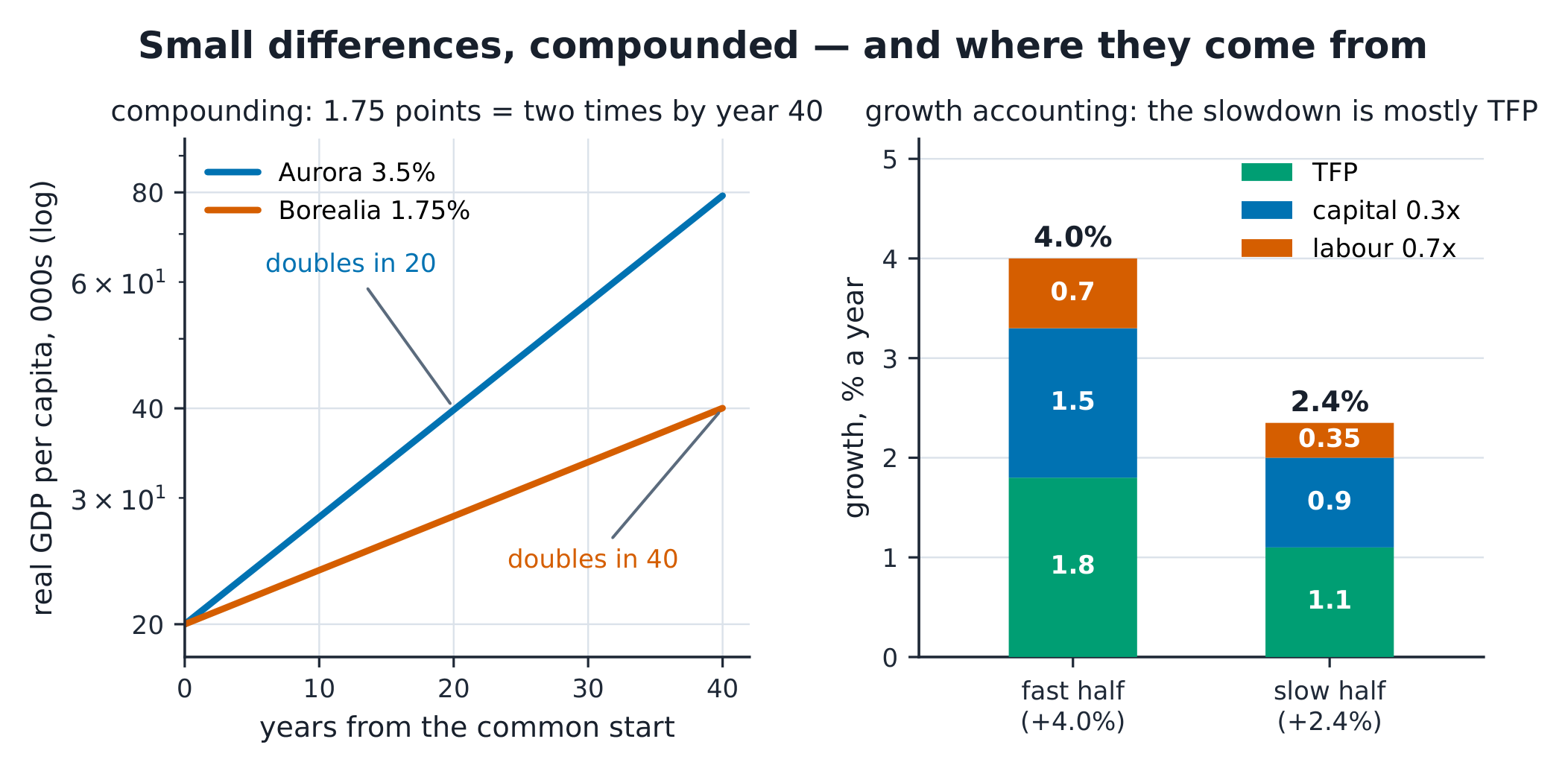
The definitions. Capital 资本 is produced means of production; the exponent 0.3 is capital's income share. Labour 劳动 force growth matters through participation and hours, not just population. The rule of 70 70法则: at g% a year, something doubles in about 70/g years. Proximate causes (capital, schooling) are the arithmetic; fundamental causes (institutions, geography, culture) explain why the proximate ones differ.
The derivation. Log-differentiate $Y = AK^{0.3}L^{0.7}$ and the weights are the income shares: $\Delta Y/Y = \Delta A/A + 0.3\Delta K/K + 0.7\Delta L/L$. Aurora's fast half-decade: output +4.0%, capital +5.0%, labour +1.0% → TFP = $4.0 - 1.5 - 0.7 = 1.8$%. Slow half: +2.4%, capital +3.0%, labour +0.5% → TFP = $2.4 - 0.9 - 0.35 = 1.15 \approx 1.1$%. The slowdown is one third fewer machines, two thirds less improvement.
Worked example 1 — the decomposition. A minister claims the fast years came from investment. The ledger says: of the 4.0%, capital deepening delivered 1.5, labour 0.7, TFP 1.8 — more than half the growth was doing things better, not owning more things. And check the logic both ways: TFP is a RESIDUAL — whatever growth is left after inputs — so measurement error in K or L lands in A and in no one's confession.
Worked example 2 — escalate to compounding. Two neighbours both start at real GDP per capita of 20,000. Aurora compounds at 3.5%; Borealia at 1.75%. Rule of 70: Aurora doubles in 20 years, Borealia in 40. After 40 years: $20{,}000 \times 2^2 = 80{,}000$ against $20{,}000 \times 2 = 40{,}000$. A 1.75-point gap, held for one working life, becomes a two-times living standard. This is why growth policy dwarfs every business-cycle debate.
Common mistakes. Reading TFP as "technology only" — it is everything inputs fail to explain, including mismanagement and measurement. Comparing growth rates over different windows without saying so. And extrapolating the fast phase forever — convergence is conditional, not automatic.
Summary. Growth = inputs weighted by income shares + the residual. The rule of 70 turns rates into doublings. Fundamental causes decide the long run; the residual keeps the discipline honest.
Inflation and unemployment
Why it matters. Inflation is the tax nobody voted for; unemployment is the waste nobody booked. Reading a price index and a jobs report correctly is a civic skill, and the trade-off between the two is the oldest argument in macro.
The idea, with a picture. A consumer price index 消费者价格指数 prices a FIXED basket: 10 loaves, a month of rent, 40 bus rides. If the basket cost £920 last year and £975 this year, the index reads 106.0 and inflation is 6.0% — with rent contributing 5.2 of the 6 points. An index is only as honest as its basket weights.

The definitions. Inflation 通货膨胀 is the rate of change of a price index; the deflator covers all GDP, the CPI a household basket. The Fisher equation 费雪方程: real rate = $(1+i)/(1+\pi) - 1$. The unemployment rate 失业率 = unemployed/labour force; a person is unemployed only if seeking work — discouragement shrinks the rate without creating a job. Phillips curve 菲利普斯曲线: $\pi = \pi^e - 0.8(u - u^n)$ with natural rate $u^n = 5$%.
The derivation. The basket: bread $10 \times (2.2 - 2.0) = +2$; rent $1 \times (848 - 800) = +48$; bus $40 \times (2.625 - 2.5) = +5$; total +55 on a base of 920 → CPI 106.0, inflation 6.0%, and rent's share $48/920 = 5.22$ points of it ✓. Fisher: at 5% nominal and 3% inflation the real rate is $1.05/1.03 - 1 = 1.94$% — not the naive 2%. Phillips with $\pi^e = 4$: u = 7 → $\pi = 2.4$; u = 5 → 4.0; u = 3 → 5.6 — each point of unemployment below 5 buys 0.8 of inflation, until expectations catch up.
Worked example 1 — the index under the headline. Aurora's 2022 headline: 6.0%. A tenant reads "rent rose 6%" — false: the BASKET rose 6%, of which rent contributed 5.22 points; rent itself rose $48/800 = 6.0$%, bread 10.0%, bus fares 5.0%. Weights turn item rates into basket rates: $0.022 + 5.217 \times \frac{800}{920}$… the exact statement is $\pi = \sum w_i \pi_i$ with $w_i$ the basket shares: bread 2.17% weight × 10.0%, rent 86.96% × 6.0%, bus 10.87% × 5.0% → 0.22 + 5.22 + 0.54 = 5.98 ≈ 6.0 ✓ (rounding the last point).
Worked example 2 — escalate to the Fisher trap. A saver takes a 5% deposit rate expecting 3% inflation: the ex-ante real return is 1.94%. If inflation turns out to be 6%, the ex-post real rate is $1.05/1.06 - 1 = -0.94$% — the saver paid for the surprise, the borrower gained, and the contract was silent about it. That redistribution is why central banks target stability rather than zero: an EXPECTED inflation is a tax known in advance; an unexpected one is a lottery.
Common mistakes. "The CPI went up 106%" — the index LEVEL rose from 100 to 106; inflation was 6%. Subtracting inflation from the nominal rate (the 2% error at moderate rates, worse when rates rise). And reading a falling unemployment rate as pure good news without checking participation.
Summary. Index = fixed basket priced twice; contributions are weighted item rates. Real = $(1+i)/(1+\pi) - 1$. Phillips trades inflation against unemployment only until expectations move.
Money and banking
Why it matters. Banks do not store money; they create it by lending, and the central bank steers the whole system with a handful of tools. Every mortgage rate and every bank run lives inside this machinery.
The idea, with a picture. A deposit is both a liability (the bank owes you) and the raw material of lending. With a 10% reserve ratio 存款准备金率 and no cash drain, £100 of reserves supports £1,000 of deposits: the money multiplier 货币乘数 at work, balance sheet by balance sheet.

The definitions. M1/M2 money aggregates: currency plus deposits of increasing breadth. The multiplier with cash drain $c$ and reserve ratio $r_d$: $m = (1+c)/(r_d + c)$. Central-bank tools: the policy rate, open-market operations, reserve requirements, and the lending facility — the floor system in one sentence. Nominal vs real rates is the Fisher equation of unit 4.3; the central bank moves the nominal short rate, and the economy responds to the real one.
The derivation. The chain: bank receives 100, keeps 10, lends 90; the 90 returns as a deposit, 9 is kept, 81 lent… total deposits $= 100 \times 1/(1-0.9) = 1{,}000$ ✓. With households holding cash of 30 cents per deposit dollar ($c = 0.3$): $m = 1.3/0.4 = 3.25$, so the same 100 of respires supports $325$ of money — the drain is why multipliers in real economies are 3-ish, not 10.
Worked example 1 — three balance sheets. Round 1: reserves +100, deposits +100; lend 90 → borrower spends; the seller deposits 90. Round 2: reserves +90, deposits +90; lend 81. Round 3: lend 72.9. After three rounds deposits are 100 + 90 + 81 = 271 and the chain continues to 1,000 — check the remaining 729 is $810/(1-0.9)$, the tail of the geometric series ✓. Nothing here is a vault being emptied; every loan CREATES its own deposit.
Worked example 2 — escalate to transmission. The central bank raises the policy rate from 5% to 6%. Transmission: banks' funding costs rise → lending rates rise → the real rate (expected inflation 4%) rises from 0.96% to 1.92% → investment and durable spending fall → output gap negative → inflation drifts down — each arrow a mechanism with a lag, and each lag a reason policy acts on forecasts, not readings. With the multiplier at 3.25, a 10 open-market SALE drains $32.5$ of money — tools are interlocking, not independent.
Common mistakes. "Banks lend out reserves" — lending creates deposits; reserves settle payments between banks. Confusing the multiplier's arithmetic limit with the system's behaviour (banks lend when profitable loans exist, not automatically). And quoting nominal rates as if they were the cost of borrowing.
Summary. $m = (1+c)/(r_d+c)$; deposits are created by lending. Policy rate → real rate → spending → inflation, all with lags.
Macroeconomic policy
Why it matters. When a recession hits, somebody decides. This unit is about what the decision-makers can see, what they can move, and when their answer arrives — the multiplier arithmetic and the lags, with the model's limits stated as part of the answer.
The idea, with a picture. In the simple Keynesian cross, spending multiplies: with marginal propensity to consume 边际消费倾向 $MPC = 0.75$, the multiplier 乘数 is $1/(1-0.75) = 4$. A £40bn spending rise lifts income by £160bn — but the picture's static arrow hides the clock.
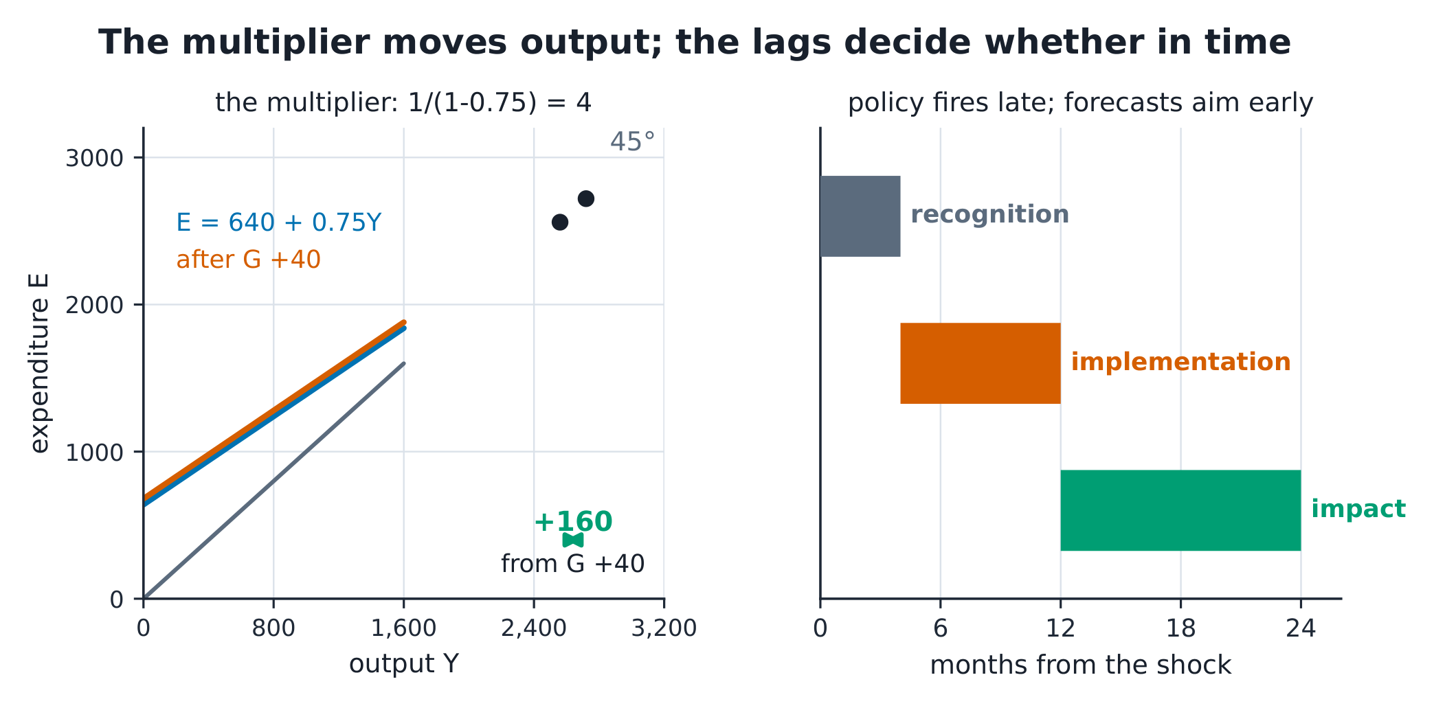
The definitions. The spending multiplier 支出乘数 is $1/(1-MPC)$; the tax multiplier is $-MPC/(1-MPC)$; the balanced-budget multiplier is exactly 1. Crowding out 挤出效应: government borrowing raises rates and displaces private investment — the multiplier's fine print. Lags: recognition (seeing the shock), implementation (passing and executing), impact (the multiplier working through) — monetary policy is quicker to fire and slower to land than fiscal.
The derivation. $MPC = 0.75$: spending multiplier $1/0.25 = 4$ ✓; $G + 40 \to Y + 160$. Tax cut $T = 40$: first-round spending is only the spent part, $40 \times 0.75 = 30$, so $\Delta Y = 30 \times 4 = 120$ ✓ — the tax multiplier is $-3$. Equal rises in G and T: $+50 \times 4$ and $-50 \times 3$ net to exactly $+50$ — the balanced-budget multiplier of 1, a rare theorem you can prove in one line.
Worked example 1 — the recession response. Aurora's output gap is −60bn. Options: G +15 (impact +60, adds to debt), T −20 (impact +60, costs 80 of revenue), or a mix. Each closes the gap arithmetically; the choice is about debt, composition and speed. Now the fine print: if the central bank simultaneously raises rates to defend inflation, part of the 60 is crowded out; if imports leak, the multiplier is smaller than 4 — the model's limits belong in the answer, not a footnote.
Worked example 2 — escalate to the dated episode. The 2021–23 global inflation: supply shocks (energy, shipping) met stimulus-strengthened demand; UK CPI peaked at 11.1% in October 2022 (ONS series), unemployment stayed near 3.7–4.0%, and central banks raised policy rates from near zero to 4–5% through 2023. Read it with this course's tools: a negative supply shock moves inflation AND output the wrong way at once (the Phillips trade-off temporarily fails), lags meant the tightening landed in 2023, and fiscal support for energy bills worked THROUGH prices, not around them. One episode, every unit of this course.
Common mistakes. Quoting the multiplier as a fact rather than a model result (leakages make real ones smaller). Comparing a tax cut and a spending rise pound-for-pound (the first round differs). And treating "policy responded" as "policy worked" without asking when the effect landed.
Summary. Multipliers: spending $1/(1-MPC)$, tax $-MPC/(1-MPC)$, balanced budget exactly 1. Lags are why policy targets forecasts; limits are part of the answer.
International linkages
Why it matters. Aurora imports a fifth of its GDP, its currency floats and its firms borrow abroad. The balance of payments is the place where domestic policy and the rest of the world settle their accounts — and where a current-account deficit is a DECISION, not a sin.
The idea, with a picture. The balance of payments 国际收支平衡表 always balances: the current account 经常账户 (trade in goods and services, net income, net transfers) is mirrored by the capital and financial account — a deficit on one is a surplus on the other, which is the same as saying the country is borrowing from abroad.
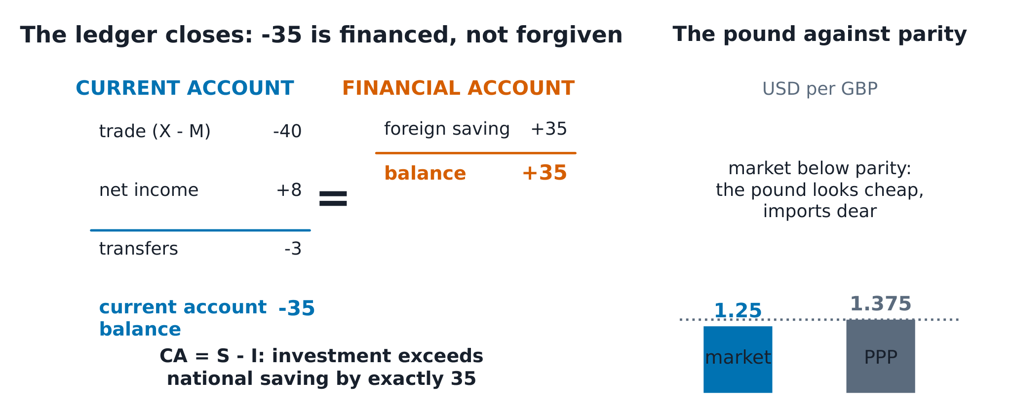
The definitions. The nominal exchange rate 汇率 is the price of one currency in another; the real exchange rate adjusts for price levels. Purchasing power parity 购买力平价 says the rate should equal the ratio of basket prices. Uncovered interest parity 未抛补利率平价: the currency with the higher interest rate is expected to depreciate, $ceteris paribus$.
The derivation. Aurora's external ledger (£bn): exports 160, imports 200 → net exports −40; net investment income +8; net transfers −3 → current account −35, matched by a financial account +35 — national accounts arithmetic again: $CA = S - I$, so a −35 current account means domestic investment exceeds national saving by exactly 35. PPP: the same basket costs 800 in pounds at home and 1,100 in dollars abroad → PPP rate $1{,}100/800 = 1.375$ USD/GBP; the market rate at 1.25 makes the pound CHEAP relative to parity — foreign goods look expensive to Aurora's consumers, exactly the force that narrows the trade gap.
Worked example 1 — the ledger closes. An Aurora journalist writes "our trade deficit is £40bn and the balance of payments must be in deficit". Both halves are wrong: the trade balance is −40, but the current account is −35 (income and transfers cut in), and the BALANCE of payments is zero by construction — the −35 is financed by a +35 financial surplus, i.e. foreign saving. The decision to worry or not is about WHAT the borrowing buys (investment versus consumption), not the sign.
Worked example 2 — escalate to parity. Aurora's rate is 1.25 while PPP says 1.375: at the margin, shopping abroad is dear, exports are cheap, and the gap should close — but slowly, because baskets are not identical and transport is real. Interest rates: Aurora 5%, the world 4%. UIP says the pound must be expected to depreciate about 1%: $1.25 \times 1.04/1.05 = 1.238$ — a saver choosing between the two currencies is, by the parity logic, indifferent once the expected move is priced. Check it like everything else in this course: the equation is a model with famous failures; carry-trade profits exist because UIP fails in the short run.
Common mistakes. Adding current and capital accounts and expecting a deficit (the sum is identically zero). Calling a depreciation bad for everyone (exporters gain; importers pay). And treating PPP as a forecast — it is a long-run anchor with decades of patience.
Summary. The BOP balances by definition; CA = S − I is the content. PPP is the long-run anchor, UIP the short-run model — both with stated limits.