跳到主要内容

多项式函数与有理函数

AP 微积分预备 · 知识点 1

本主题的视频课程 打开视频页面
17:14

多项式与有理函数

观察这条曲线。它上升,然后下降,再上升——这些是它的极值点。它穿过水平轴——这些是根,即…

英语旁白 · 英中内嵌字幕

1.1

协同变化

教学大纲

学习目标 1.1.A: 通过比较函数值,描述函数的输入值和输出值如何协同变化。

  • 1.1.A.1 函数是一种数学关系,它将一组输入值映射到一组输出值,使得每个输入值恰好对应一个输出值。输入值的集合称为函数的定义域,输出值的集合称为函数的值域。表示输入值的变量称为自变量,表示输出值的变量称为因变量。
  • 1.1.A.2 函数的输入值和输出值按照函数法则协同变化,该法则可以通过图形、数值、解析或语言方式表达。
  • 1.1.A.3 如果随着输入值的增加,输出值始终增加,则称函数在其定义域的某个区间上是递增的。即对于区间内的所有 $a$ 和 $b$,若 $a < b$,则 $f(a) < f(b)$。
  • 1.1.A.4 如果随着输入值的增加,输出值始终减少,则称函数在其定义域的某个区间上是递减的。即对于区间内的所有 $a$ 和 $b$,若 $a < b$,则 $f(a) > f(b)$。

学习目标 1.1.B: 构建图表来表示情境中两个相互依赖变化的量。

  • 1.1.B.1 函数的图象显示了一组输入-输出对,并展示了函数输入值和输出值的变化情况。
  • 1.1.B.2 用语言描述现象各部分如何共同变化,可以作为构建图表的基础。
  • 1.1.B.3 当变化率增加时,函数的图象在相应区间内是向上凹(开口向上)的。
  • 1.1.B.4 当变化率减少时,函数的图象在相应区间内是向下凹(开口向下)的。
  • 1.1.B.5 当输出值为零时,图象与 $x$ 轴相交。对应的输入值被称为函数的零点。
来源:College Board AP 课程与考试说明

English

A function 函数 is a rule that maps each input to exactly one output. The set of allowed inputs is the domain 定义域; the set of outputs is the range 值域. The input variable is the independent variable 自变量 and the output variable is the dependent variable 因变量. A function rule can be shown graphically, numerically, analytically (a formula), or verbally.

As the input changes, the output changes "in tandem" – together. Over an interval, a function is:

  • increasing 递增 if, whenever $a<b$, then $f(a)<f(b)$ (bigger input, bigger output);
  • decreasing 递减 if, whenever $a<b$, then $f(a)>f(b)$ (bigger input, smaller output).

A graph of a function shows all its input–output pairs, so you can read this behavior straight off the picture.

探索

观察两个量同时变化

y = ax² + bx + c

预备微积分研究输出如何与输入同步变化。从左到右阅读曲线:在陡峭处,$y$对$x$的小变化产生大幅变化;在平坦处,$y$几乎不动。

词汇 训练
English 中文 拼音
function/ˈfʌŋkʃn/ 函数 hán shù
domain/dəˈmeɪn/ 定义域 dìng yì yù
range/reɪndʒ/ 值域 zhí yù
independent variable/ˌɪndɪˈpendənt ˈveərɪəbl/ 自变量 zì biàn liàng
dependent variable/dɪˈpendənt ˈveərɪəbl/ 因变量 yīn biàn liàng
increasing/ɪnˈkriːsɪŋ/ 递增 dì zēng
decreasing/ˈdiːkriːsɪŋ/ 递减 dì jiǎn
1.2

变化率

教学大纲

学习目标 1.2.A: 利用点附近的平均变化率比较两点的变化率。

  • 1.2.A.1 函数在其定义域某个区间上的平均变化率,是指产生与函数在该区间上输出值变化量相同的常量变化率。它是该区间上输出值的变化量与输入值的变化量的比值。
  • 1.2.A.2 函数在某一点的变化率量化了当输入值在该点发生变化时,输出值发生变化的速率。如果存在这样的值,则可以通过包含该点的较小区间上的函数平均变化率来近似该点的变化率。
  • 1.2.A.3 如果存在这样的值,可以通过包含每一点的足够小区间上的平均变化率近似值来比较两点的变化率。

学习目标 1.2.B: 描述两个数量在函数的不同点和不同区间内如何共同变化。

  • 1.2.B.1 变化率量化了两个数量是如何共同变化的。
  • 1.2.B.2 正的变化率表明当一个数量增加或减少时,另一个数量也做同样的变化(即同向变化)。
  • 1.2.B.3 负的变化率表明当一个数量增加时,另一个数量减少。

来源:College Board AP 课程与考试说明

English

The average rate of change 平均变化率 of a function over an interval is the change in output divided by the change in input – the single constant rate that would give the same total change. Over $[a,b]$:

$$\text{avg rate} = \frac{f(b)-f(a)}{b-a}.$$

The rate of change at a point measures how fast the output changes right at that input. You approximate it with average rates over small intervals around the point. Comparing two points, the one with the larger average rate (over small enough intervals) is changing faster. A positive rate means both quantities move the same way; a negative rate means they move in opposite ways.

Worked example. For $f(x)=x^2$, the average rate of change over $[1,4]$ is $\dfrac{f(4)-f(1)}{4-1}=\dfrac{16-1}{3}=5$. Over $[1,2]$ it is $\dfrac{4-1}{1}=3$ – the rate itself changes, which is exactly why $f$ is not linear.

探索

让区间不断缩小,割线就变成了切线

f(x) = 0.5x²

拖动这个点,读出某一点处的斜率——这就是区间缩小到零时平均变化率的极限。

词汇 训练
English 中文 拼音
average rate of change/ˈævrɪdʒ reɪt ɒv tʃeɪndʒ/ 平均变化率 píng jūn biàn huà lǜ
1.3

线性函数与二次函数的变化率

教学大纲

学习目标 1.3.A: 确定数列和函数的平均变化率,包括线性函数、二次函数及其他类型的函数。

  • 1.3.A.1 对于线性函数,在任意长度的输入值区间上,其平均变化率是恒定的。
  • 1.3.A.2 对于二次函数,在连续等长输入值区间上的平均变化率可以由一个线性函数来表示。
  • 1.3.A.3 在闭区间 $[a, b]$ 上的平均变化率即为连接点 $(a, f(a))$ 与点 $(b, f(b))$ 的割线的斜率。

学习目标 1.3.B: 确定线性函数、二次函数及其他类型函数的平均变化率的变化情况。

  • 1.3.B.1 对于线性函数,由于其在连续等长输入值区间上的平均变化率可由一个常数函数表示,因此这些平均变化率以零的速率变化(即保持不变)。
  • 1.3.B.2 对于二次函数,由于其在连续等长输入值区间上的平均变化率可由一个线性函数表示,因此这些平均变化率以恒定的速率变化。
  • 1.3.B.3 当所有短长度输入值区间上的平均变化率均递增时,该函数的图像向上凹(开口向上);当所有短长度输入值区间上的平均变化率均递减时,该函数的图像向下凹(开口向下)。

来源:College Board AP 课程与考试说明

English

The average rate of change over $[a,b]$ is the slope of the secant line 割线 from $(a,f(a))$ to $(b,f(b))$.

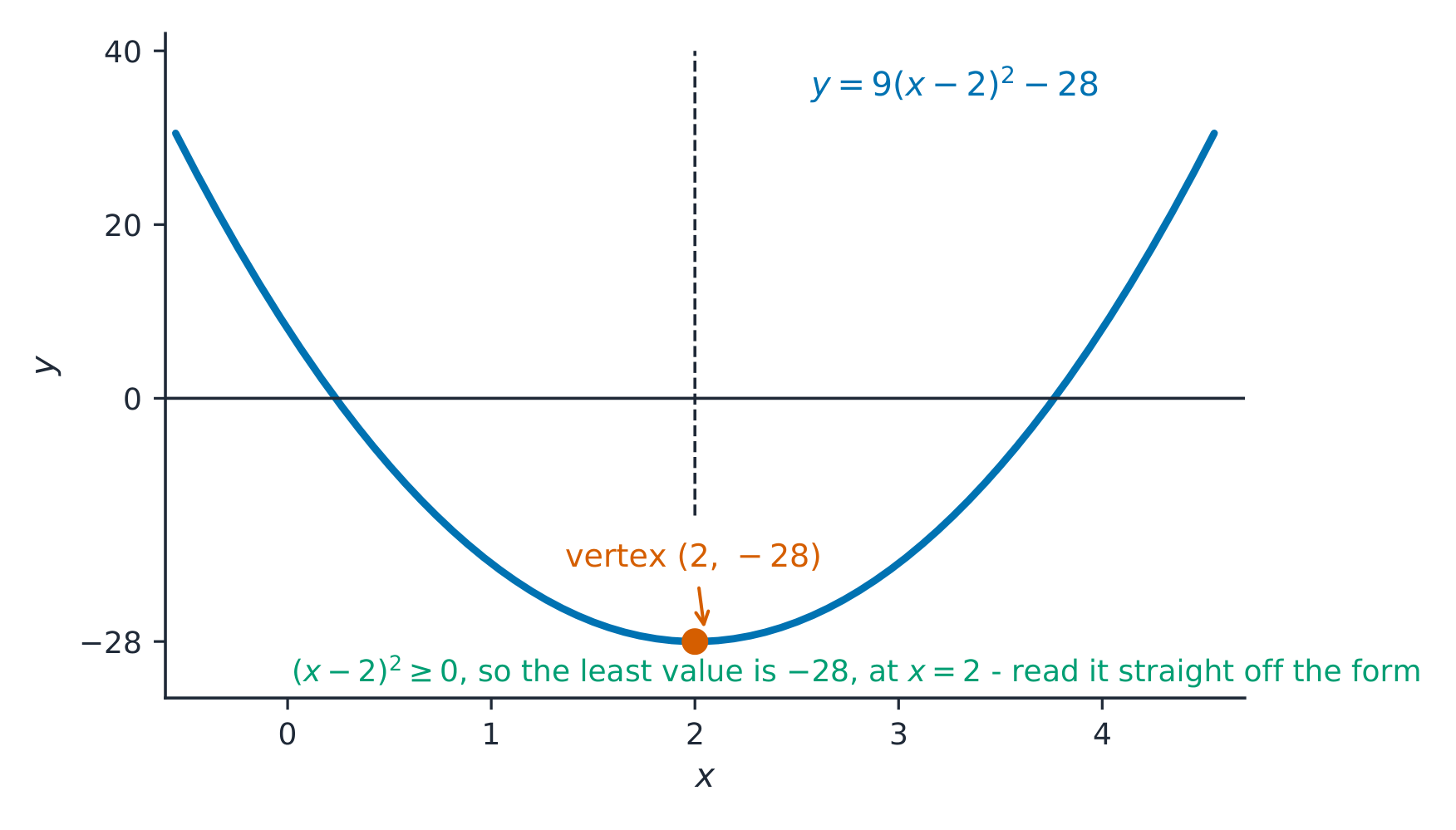
Completing the square gives the vertex of a parabola
  • For a linear 线性 function, the average rate of change over any interval is constant – so the rate at which the rate changes is zero.
  • For a quadratic 二次 function, the average rates of change over equal-length intervals themselves form a linear pattern – so those rates change at a constant rate.

This "rate of the rate" idea distinguishes function types: a constant second difference signals a quadratic.

Worked example. Which kind of function fits this table (equally spaced inputs)?

$x$ $0$ $1$ $2$ $3$ $4$
$f(x)$ $1$ $3$ $9$ $19$ $33$
1st differences $2$ $6$ $10$ $14$
2nd differences $4$ $4$ $4$

The first differences (the average rates over each step) are not constant, so $f$ is not linear. They increase by the same amount, $4$, each time, so the second differences are constant: a quadratic model fits. (In fact $f(x)=2x^2+1$.)

The Golden Gate Bridge with its curved main cable
A hanging bridge cable takes the shape of a parabola-like curve — a quadratic you can see in steel
探索

探索二次函数的变化率

y = ax² + bx + c

移动滑块并观察抛物线 tilt。其平均变化率不是恒定的——在顶点的一侧斜率为正,另一侧为负。注意$a$如何使其向上或向下开口。

词汇 训练
English 中文 拼音
secant line/ˈsiːkənt laɪn/ 割线 gē xiàn
linear/ˈlɪnɪə/ 线性 xiàn xìng
quadratic/kwɒˈdrætɪk/ 二次 èr cì
1.4

多项式函数与变化率

教学大纲

学习目标 1.4.A: 识别与变化率相关的多项式函数的关键特征。

  • 1.4.A.1 $x$ 的非常数多项式函数是指任何等价于解析形式 $p(x) = a_n x^n + a_{n-1} x^{n-1} + a_{n-2} x^{n-2} + \ldots + a_2 x^2 + a_1 x + a_0$ 的函数表示,其中 $n$ 为正整数,$a_i$ 为 $i$ 从 $1$ 到 $n$ 时的任意实数,且 $a_n$ 不为零。该多项式的次数为 $n$,首项为 $a_n x^n$,首项系数为 $a_n$。常数也是零次多项式函数。
  • 1.4.A.2 当多项式函数在递增和递减之间转换时,或在定义域受限的多项式的包含端点处,该多项式函数将具有局部或相对的最大值或最小值输出。在所有局部最大值中,最大者称为全局或绝对最大值。同样,在所有局部最小值中最小者称为全局或绝对最小值。
  • 1.4.A.3 在非常数多项式函数的每两个不同实零点之间,至少存在一个对应于局部最大值或局部最小值的输入值。
  • 1.4.A.4 偶次多项式函数将具有全局最大值或全局最小值。
  • 1.4.A.5 多项式函数的拐点出现在函数变化率由递增变为递减或由递减变为递增的输入值处。这发生在多项式函数的图像由上凸(凹向上)变为下凸(凹向下),或由下凸(凹向下)变为上凸(凹向上)的地方。

来源:College Board AP 课程与考试说明

English
A smooth bridge curve: polynomial and rational graphs model real shapes with asymptotes and turns

A nonconstant polynomial 多项式 has the form

$$p(x)=a_n x^n + a_{n-1}x^{n-1}+\cdots+a_1 x + a_0,\quad a_n\neq 0.$$
Its degree 次数 is $n$, its leading term 首项 is $a_n x^n$, and its leading coefficient 首项系数 is $a_n$. A constant is a polynomial of degree $0$.

Key features:

  • Where a polynomial switches between increasing and decreasing, it has a local (relative) extremum 局部极值. The greatest local maximum is the global (absolute) maximum 全局最大值 only when the polynomial has one — but most polynomials are unbounded (every odd-degree polynomial runs off to $\pm\infty$), so they have no global maximum or minimum at all.
  • Between any two distinct real zeros there is at least one local maximum or minimum.
  • An even-degree polynomial has either a global maximum or a global minimum.
  • A point of inflection 拐点 is where the graph changes concavity – from concave up 上凹 to concave down 下凹 or the reverse – i.e. where the rate of change switches between increasing and decreasing.
  • A function has symmetry when it is even 偶函数 – $f(-x)=f(x)$, graph symmetric across the $y$-axis (like $x^2$, $x^4$) – or odd 奇函数 – $f(-x)=-f(x)$, graph symmetric by rotation about the origin (like $x^3$, $x^5$). Test by substituting $-x$ and simplifying; later, $\cos\theta$ is even and $\sin\theta$ is odd.
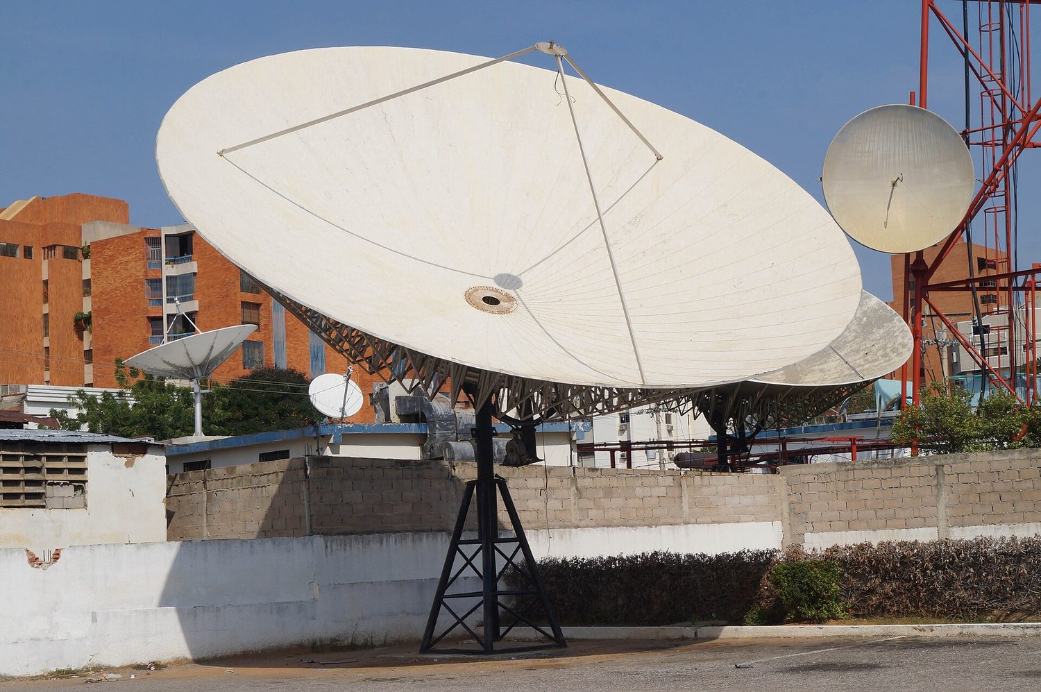
A satellite dish mounted on a wall, its curved reflector aimed at the sky with the receiver held at the focus
A satellite dish is a parabola of revolution: every parallel ray reflects to the same focus
探索

重塑一个三次函数,数一数它的转折点

y = ax³ + bx² + cx + d

Adjust the sliders. A degree-3 curve can wiggle at most twice — try to make it turn three times (you cannot).

词汇 训练
English 中文 拼音
polynomial/ˌpɒlɪˈnəʊmɪəl/ 多项式 duō xiàng shì
degree/dɪˈɡriː/ 次数 cì shù
leading term/ˈliːdɪŋ tɜːm/ 首项 shǒu xiàng
leading coefficient/ˈliːdɪŋ ˌkəʊɪˈfɪʃənt/ 首项系数 shǒu xiàng xì shù
local (relative) extremum/ˈləʊkl ekˈstreməm/ 局部极值 jú bù jí zhí
global (absolute) maximum/ˈɡləʊbl ˈmæksɪməm/ 全局最大值 quán jú zuì dà zhí
point of inflection/pɔɪnt ɒv ɪnˈflekʃn/ 拐点 guǎi diǎn
concave up/kɒnˈkeɪv ʌp/ 上凹 shàng āo
concave down/kɒnˈkeɪv daʊn/ 下凹 xià āo
even/ˈiːvən/ 偶函数 ǒu hán shù
odd/ɒd/ 奇函数 jī hán shù
1.5

多项式函数与复数零点

教学大纲

学习目标 1.5.A: 在获得适当因式分解或使用技术工具的情况下,识别与多项式函数零点相关的关键特征。

  • 1.5.A.1 如果 $a$ 是一个复数且 $p(a) = 0$,则称 $a$ 为多项式函数 $p$ 的零点,或方程 $p(x) = 0$ 的根。如果 $a$ 是实数,当且仅当 $a$ 是 $p$ 的零点时,$(x - a)$ 才是 $p$ 的一个一次因式。
  • 1.5.A.2 如果一次因式 $(x - a)$ 重复出现了 $n$ 次,则该多项式函数对应的零点的重数为 $n$。一个 $n$ 次多项式函数在计入重数的情况下恰好有 $n$ 个复数零点。
  • 1.5.A.3 如果 $a$ 是多项式函数 $p$ 的一个实数零点,那么 $y = p(x)$ 的图像在点 $(a, 0)$ 处有一个 $x$ 轴截距。因此,多项式的实数零点可以作为满足多项式不等式的区间的端点。
  • 1.5.A.4 如果 $a + bi$ 是多项式函数 $p$ 的一个非实数零点,那么其共轭 $a - bi$ 也是 $p$ 的零点。
  • 1.5.A.5 如果多项式函数的实数零点 $a$ 的重数为偶数,那么在 $x = a$ 附近的输入值所对应的输出值的符号相同。对于这些多项式函数,其图像将在 $x = a$ 处与 $x$ 轴相切。
  • 1.5.A.6 可以通过检查等间隔输入值下的输出值的连续差分来确定多项式函数的次数。多项式函数的次数等于使连续第 $n$ 阶差分保持常数的最小值 $n$。

学习目标 1.5.B: 判断多项式函数是偶函数还是奇函数。

  • 1.5.B.1 偶函数关于直线 $x = 0$ 具有图形对称性,并且在代数上具有性质 $f(-x) = f(x)$。如果 $n$ 是偶数,那么形如 $p(x) = a_n x^n$(其中 $n \geq 1$ 且 $a_n \neq 0$)的多项式是偶函数。
  • 1.5.B.2 奇函数关于点 $(0, 0)$ 具有图形对称性,并且在代数上具有性质 $f(-x) = -f(x)$。如果 $n$ 是奇数,那么形如 $p(x) = a_n x^n$(其中 $n \geq 1$ 且 $a_n \neq 0$)的多项式是奇函数。

来源:College Board AP 课程与考试说明

English

A zero 零点 (or root 根) of $p$ is a number $a$ with $p(a)=0$. For a real $a$, $(x-a)$ is a factor of $p$ exactly when $a$ is a zero. If the factor $(x-a)$ is repeated $n$ times, that zero has multiplicity 重数 $n$. Counting multiplicities, a degree-$n$ polynomial has exactly $n$ complex 复数 zeros.

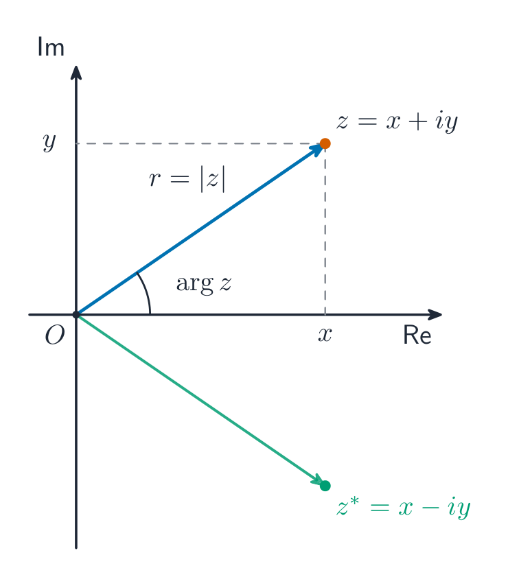
A complex number on an Argand diagram: modulus is the distance, argument the angle
  • A real zero $a$ gives an $x$-intercept at $(a,0)$; real zeros are the endpoints of the intervals where $p(x)\ge 0$ or $\le 0$.
  • Non-real zeros come in conjugate 共轭 pairs: if $a+bi$ is a zero, so is $a-bi$.
  • At a real zero of even multiplicity the graph is tangent to the $x$-axis (it touches but does not cross); at odd multiplicity it crosses.

Worked example. A cubic $p$ has a zero of multiplicity $2$ at $x=-1$, a zero at $x=3$, and $p(0)=6$. Find $p(x)$ and describe its graph.

Each zero gives a factor, so $p(x)=a(x+1)^2(x-3)$. Use the point: $p(0)=a(1)^2(-3)=-3a=6$, so $a=-2$ and

$$p(x)=-2(x+1)^2(x-3).$$

The graph touches the $x$-axis at $x=-1$ (even multiplicity) and crosses it at $x=3$. The leading term is $-2x^3$ (negative, odd degree), so $\lim_{x\to\infty}p(x)=-\infty$ and $\lim_{x\to-\infty}p(x)=\infty$.

  • The degree equals the least $n$ for which the $n$th successive differences of equally-spaced outputs become constant.
探索

一个复零点和它的镜像伙伴

画出一个零点 a + bi。对实系数多项式,它的共轭 a − bi(关于实轴的镜像)也一定是零点。

词汇 训练
English 中文 拼音
zero/ˈzɪərəʊ/ 零点 líng diǎn
root/ruːt/ 根 gēn
multiplicity/ˌmʌltɪˈplɪsɪti/ 重数 chóng shù
complex/ˈkɒmpleks/ 复数 fù shù
conjugate/ˈkɒndʒuːɡeɪt/ 共轭 gòng è
1.6

多项式函数与末端行为

教学大纲

学习目标 1.6.A: 描述多项式函数的端点行为。

  • 1.6.A.1 当非零常数多项式函数的输入值无限增大时,其输出值也会无限增大或无限减小。对应的数学符号表示为 $\lim_{x \to \infty} p(x) = \infty$ 或 $\lim_{x \to \infty} p(x) = -\infty$。
  • 1.6.A.2 当非零常数多项式函数的输入值无限减小时,其输出值也会无限增大或无限减小。对应的数学符号表示为 $\lim_{x \to -\infty} p(x) = \infty$ 或 $\lim_{x \to -\infty} p(x) = -\infty$。
  • 1.6.A.3 多项式的次数和首项的符号决定了多项式函数的端点行为,因为当输入值无限增大或减小时,首项的值会主导所有低次项的值。

来源:College Board AP 课程与考试说明

English

End behavior 末端行为 describes where a function heads as the input grows without bound. For a nonconstant polynomial, as $x\to\pm\infty$ the output goes to $+\infty$ or $-\infty$, written e.g. $\lim_{x\to\infty}p(x)=\infty$. Which way depends entirely on the leading term $a_n x^n$, because for large $|x|$ it dominates all lower-degree terms: the sign of $a_n$ and whether $n$ is even or odd fix both ends.

Every polynomial's ends are decided by its degree's parity and the sign of its leading coefficient
探索

查看首项如何决定端点行为

y = ax³ + bx² + cx + d

首项决定两端的行为。对于系数为$a>0$的三次函数,图像左侧下降右侧上升;若使$a<0$,两端互换。当$x\to\pm\infty$时,最高次幂项主导所有其他项。

词汇 训练
English 中文 拼音
End behavior/end bɪˈheɪvjə/ 末端行为 mò duān xíng wéi
1.7

有理函数与末端行为

教学大纲

学习目标 1.7.A: 描述有理函数的端点行为。

  • 1.7.A.1 有理函数以两个多项式函数的商的形式进行解析表示,它衡量了分子中的多项式函数与分母中的多项式函数在定义域内每个值处的相对大小。
  • 1.7.A.2 有理函数的端点行为受次数较高的多项式影响最大,因为其数值将在输入值绝对值较大时主导有理函数的数值。对于绝对值较大的输入值,多项式主要由其首项决定。因此,通过考察首项对应的商可以理解有理函数的端点行为。
  • 1.7.A.3 如果对于绝对值较大的输入值,分子中的多项式主导分母中的多项式,那么首项的商是一个非恒定多项式,且原有理函数具有该多项式的端点行为。如果该多项式是线性的,则有理函数的图像具有一条与该直线平行的斜渐近线。
  • 1.7.A.4 如果对于绝对值较大的输入值,有理函数中的两个多项式互不主导,那么首项的商是一个常数,该常数指示了原有理函数图像的水平渐近线位置。
  • 1.7.A.5 如果对于绝对值较大的输入值,分母中的多项式主导分子中的多项式,那么首项的商是一个分子为常数、分母为非恒定多项式的有理函数,且原有理函数的图像在 $y = 0$ 处有一条水平渐近线。
  • 1.7.A.6 当有理函数 $r$ 的图像在 $y = b$ 处有一条水平渐近线(其中 $b$ 为常数)时,随着输入值无界增加或减少,有理函数的输出值会任意接近 $b$ 并保持任意接近 $b$。相应的数学符号表示为 $\lim_{x \to \infty} r(x) = b$ 或 $\lim_{x \to -\infty} r(x) = b$。

来源:College Board AP 课程与考试说明

English

A rational function 有理函数 is a quotient of two polynomials, $r(x)=\dfrac{\text{numerator}}{\text{denominator}}$. Its end behavior is governed by the quotient of the leading terms:

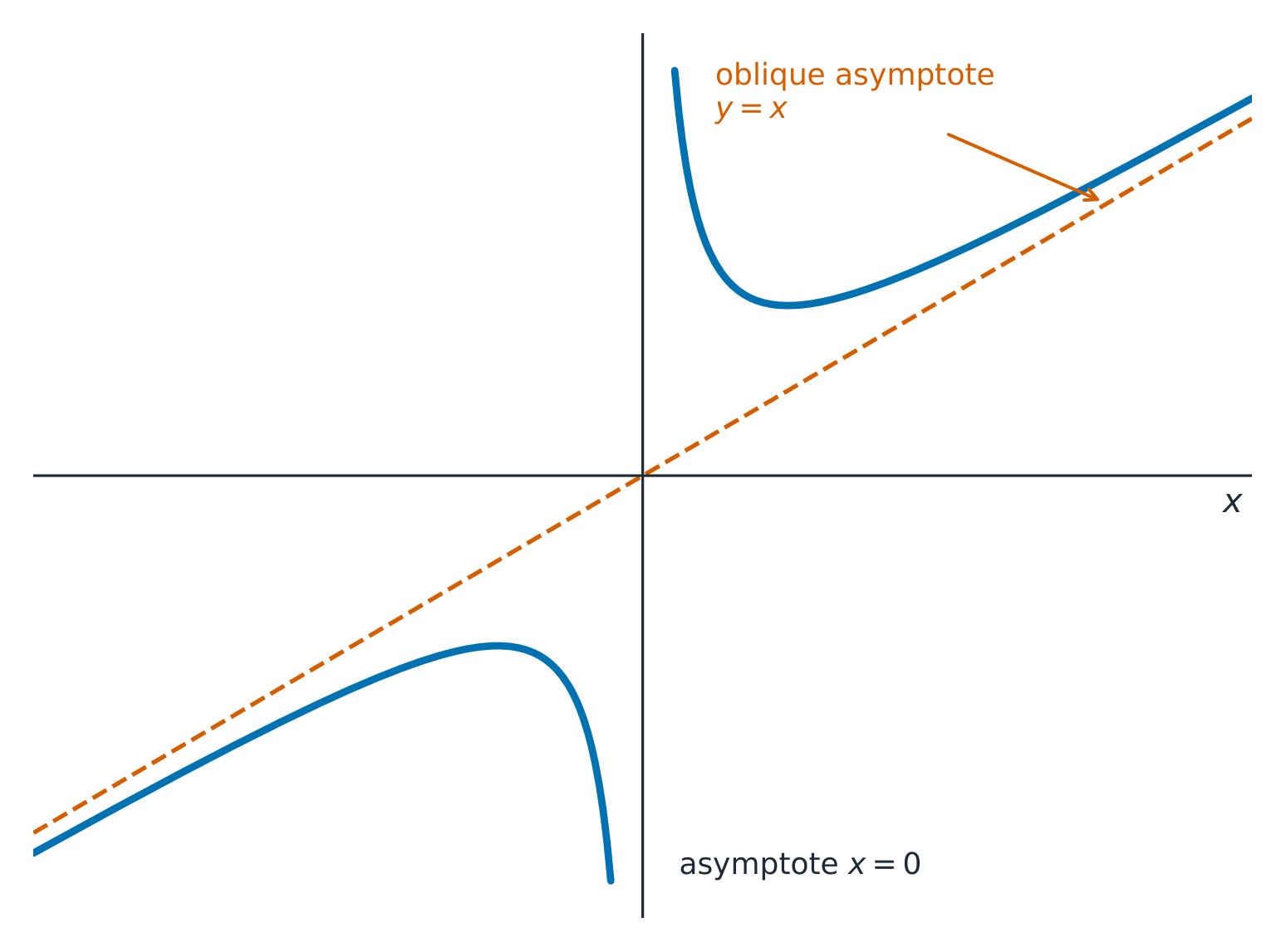
When the numerator has higher degree, the curve approaches a slanting asymptote
  • Numerator degree > denominator degree: the quotient is a nonconstant polynomial, and $r$ follows that polynomial's end behavior. If that quotient is linear, the graph has a slant asymptote 斜渐近线.
  • Equal degrees: the quotient is a constant, giving a horizontal asymptote 水平渐近线 $y=$ the ratio of leading coefficients.
  • Numerator degree < denominator degree: the quotient tends to $0$, so the horizontal asymptote is $y=0$.

At a horizontal asymptote $y=b$, the outputs get and stay arbitrarily close to $b$: $\lim_{x\to\pm\infty}r(x)=b$.

探索

上下滑动水平渐近线

y = a/(x − b) + c

改变 c,整条曲线在远处就会稳定在新的高度 y = c——那条水平线就是末端行为。

词汇 训练
English 中文 拼音
rational function/ˈræʃənl ˈfʌŋkʃn/ 有理函数 yǒu lǐ hán shù
slant asymptote/slænt ˈæsɪmptəʊt/ 斜渐近线 xié jiàn jìn xiàn
horizontal asymptote/ˌhɒrɪˈzɒntl ˈæsɪmptəʊt/ 水平渐近线 shuǐ píng jiàn jìn xiàn
1.8

有理函数与零点

教学大纲

学习目标 1.8.A: 确定有理函数的零点。

  • 1.8.A.1 有理函数的实零点对应于其分子在定义域内的实零点。
  • 1.8.A.2 有理函数 $r$ 的多项式函数的实零点是不等式 $r(x) \geq 0$ 或 $r(x) \leq 0$ 所满足区间的端点或渐近线。

来源:College Board AP 课程与考试说明

English

The real zeros of a rational function are the real zeros of its numerator that are still in the domain. These zeros, together with the zeros of the denominator, split the number line into the intervals you test when solving inequalities $r(x)\ge 0$ or $r(x)\le 0$.

Worked example. Solve $\dfrac{x-2}{x+1}\ge 0$. The numerator is zero at $x=2$ and the denominator at $x=-1$. Test one value in each interval:

Interval $x<-1$ $-1<x<2$ $x>2$
Test value $x=-2$: $\tfrac{-4}{-1}=4$ $x=0$: $\tfrac{-2}{1}=-2$ $x=3$: $\tfrac{1}{4}$
Sign $+$ $-$ $+$

So $x<-1$ or $x\ge 2$. Include $x=2$ (the value $0$ is allowed) but never $x=-1$, where $r$ is undefined.

探索

它在哪里穿过,又在哪里断开?

y = a/(x − b) + c

曲线在它的零点处穿过 x 轴,却在 x = b(分母为零)处断开。这是两个不同的地方。

1.9

有理函数与竖直渐近线

教学大纲

学习目标 1.9.A: 确定有理函数图像的垂直渐近线。

  • 1.9.A.1 如果 $a$ 是有理函数分母中多项式函数的实零点,且不是分子中多项式函数的实零点,则该有理函数的图像在 $x = a$ 处有一条垂直渐近线。此外,如果 $a$ 作为分母中的实零点的重数大于其作为分子中的实零点的重数,则在 $x = a$ 处也存在垂直渐近线。
  • 1.9.A.2 在有理函数的垂直渐近线 $x = a$ 附近,分母中多项式函数的值任意接近于零,因此有理函数 $r$ 的值会无限增大或减小。对应的数学符号表示为:对于接近 $a$ 且大于 $a$ 的输入值,$\lim_{x \to a^+} r(x) = \infty$ 或 $\lim_{x \to a^+} r(x) = -\infty$;对于接近 $a$ 且小于 $a$ 的输入值,$\lim_{x \to a^-} r(x) = \infty$ 或 $\lim_{x \to a^-} r(x) = -\infty$。

来源:College Board AP 课程与考试说明

English

A vertical asymptote 垂直渐近线 occurs at $x=a$ when $a$ is a zero of the denominator but not cancelled by the numerator – more precisely, when its multiplicity in the denominator exceeds its multiplicity in the numerator. Near it, the denominator is nearly zero, so $r$ shoots to $\pm\infty$: $\lim_{x\to a^{\pm}}r(x)=\pm\infty$. Check each side, since the two sides can go opposite ways.

Worked example. Describe $r(x)=\dfrac{2x^2+3}{x^2-1}$. The numerator and denominator have equal degree, so the horizontal asymptote is $y=\dfrac{2}{1}=2$. The denominator $x^2-1$ is zero at $x=\pm1$ and neither cancels, so there are vertical asymptotes at $x=1$ and $x=-1$.

A rational function approaching a vertical asymptote and a horizontal asymptote
探索

探索垂直渐近线

y = a/(x − b) + c

这是 $y = \dfrac{a}{x-b} + c$。图像朝 急剧上升,在 处出现 垂直渐近线(分母为零),并逐渐趋近于 水平渐近线 。滑动 和 以移动每条直线。 $\pm\infty$ 在 垂直渐近线 竖直渐近线 $x = b$ (底部为零)并趋于平缓至 水平渐近线 水平渐近线 $y = c$. 滑动 $b$ 和 $c$ 移动每一行。

词汇 训练
English 中文 拼音
vertical asymptote/ˈvɜːtɪkl ˈæsɪmptəʊt/ 垂直渐近线 chuí zhí jiàn jìn xiàn
1.10

有理函数与空洞

教学大纲

学习目标 1.10.A: 确定有理函数图像中的可去间断点。

  • 1.10.A.1 如果分子中某个实零点的重数大于或等于其在分母中的重数,则该有理函数的图像在对应的输入值处存在一个可去间断点。
  • 1.10.A.2 如果有理函数 $r$ 的图像在 $x = c$ 处存在一个可去间断点,则该间断点的位置可以通过考察足够接近 $c$ 的输入值所对应的输出值来确定。如果足够接近 $c$ 的输入值对应的输出值任意接近于 $L$,则该间断点位于坐标为 $(c, L)$ 的点处。相应的数学符号表示为 $\lim_{x \to c} r(x) = L$。需要注意的是,$\lim_{x \to c^-} r(x) = \lim_{x \to c^+} r(x) = \lim_{x \to c} r(x) = L$。

来源:College Board AP 课程与考试说明

English

A hole 空洞 (removable point) occurs at $x=c$ when a factor cancels – the multiplicity of the zero $c$ in the numerator is at least its multiplicity in the denominator. The graph is missing a single point. Its height is the limit of the simplified function: if inputs near $c$ give outputs near $L$, the hole is at $(c,L)$, and $\lim_{x\to c}r(x)=L$.

Worked example. Find all the key features of $r(x)=\dfrac{x^2-4}{x^2-x-2}$. Factor first:

$$r(x)=\frac{(x-2)(x+2)}{(x-2)(x+1)}=\frac{x+2}{x+1}\quad (x\neq 2).$$
  • Hole at $x=2$: the factor $(x-2)$ cancels. Its height comes from the simplified form, $\tfrac{2+2}{2+1}=\tfrac43$, so the hole is at $\left(2,\tfrac43\right)$.
  • Vertical asymptote $x=-1$: a zero of the denominator that does not cancel.
  • Zero at $x=-2$, so the $x$-intercept is $(-2,0)$.
  • Horizontal asymptote $y=1$: equal degrees, leading coefficients $\tfrac11$.

A common error is to call $x=2$ a vertical asymptote because it makes the original denominator zero: check whether the factor cancels first.

探索

化简后的函数只是一条直线——但少了一个点

y = ax + b

这是 (x²−1)/(x−1) 的化简形式。图像是直线 y = x + 1,但真正的函数在 x = 1 处有一个空心,因为原式在那里无定义。

词汇 训练
English 中文 拼音
hole/həʊl/ 空洞 kōng dòng
1.11

多项式与有理表达式的等价表示

教学大纲

学习目标 1.11.A: 将多项式和有理表达式改写为等价形式。

  • 1.11.A.1 由于多项式或有理函数的因式分解形式能直接提供实数零点的信息,因此它可以揭示关于 $x$ 轴截距、渐近线、可去间断点(空洞)、定义域和值域的信息。
  • 1.11.A.2 多项式或有理函数的标准形式可以揭示函数的端点行为(末项行为)。
  • 1.11.A.3 从同一多项式或有理函数的不同分析表示中提取的信息可用于回答情境中的问题。

学习目标 1.11.B: 使用长除法确定两个多项式函数的商。

  • 1.11.B.1 多项式长除法是一种代数过程,类似于涉及商和余数的数值长除法。如果用多项式 $g$ 除多项式 $f$,则 $f$ 可以重写为 $f(x) = g(x)q(x) + r(x)$,其中 $q$ 是商,$r$ 是余数,且 $r$ 的次数小于 $g$ 的次数。
  • 1.11.B.2 多项式长除法的结果有助于求有理函数图像的斜渐近线方程。

学习目标 1.11.C: 使用二项式定理改写二项式的重复乘积。

  • 1.11.C.1 二项式定理利用帕斯卡三角形(杨辉三角)中某一行的条目,可以更轻松地展开形如 $(a + b)^n$ 的表达式,包括形如 $p(x) = (x + c)^n$ 的多项式函数,其中 $c$ 为常数。

来源:College Board AP 课程与考试说明

English

The same expression, written differently, reveals different features:

  • Factored form shows real zeros, and hence $x$-intercepts, holes, vertical asymptotes, and domain.
  • Standard form (expanded) shows the degree and leading term, and hence end behavior.

Polynomial long division 多项式长除法 rewrites $f(x)=g(x)\,q(x)+r(x)$, where $q$ is the quotient 商 and $r$ the remainder 余数 (of smaller degree than $g$). The quotient gives the equation of a slant asymptote when the numerator's degree is one more than the denominator's.

Worked example. Divide: $x^2+3x+5=(x+1)(x+2)+3$, so

$$\frac{x^2+3x+5}{x+1}=x+2+\frac{3}{x+1}.$$

As $x\to\pm\infty$ the remainder term $\tfrac{3}{x+1}$ tends to $0$, so the graph approaches the slant asymptote $y=x+2$.

词汇 训练
English 中文 拼音
Polynomial long division/ˌpɒlɪˈnəʊmɪəl lɒŋ dɪˈvɪʒn/ 多项式长除法 duō xiàng shì zhǎng chú fǎ
quotient/ˈkwəʊʃənt/ 商 shāng
remainder/rɪˈmeɪndə/ 余数 yú shù
1.12

函数的变换

教学大纲

学习目标 1.12.A: 构造一个作为另一函数的加法和/或乘法变换的函数。

  • 1.12.A.1 函数 $g(x) = f(x) + k$ 是函数 $f$ 的加法变换,其结果是将 $f$ 的图像沿垂直方向平移 $k$ 个单位。
  • 1.12.A.2 函数 $g(x) = f(x + h)$ 是函数 $f$ 的加法变换,其结果是将 $f$ 的图像沿水平方向平移 $-h$ 个单位。
  • 1.12.A.3 函数 $g(x) = a f(x)$(其中 $a \neq 0$)是函数 $f$ 的乘法变换,其结果是将 $f$ 的图像进行垂直方向的伸缩,伸缩因子为 $|a|$。如果 $a < 0$,该变换还涉及关于 $x$ 轴的反射。
  • 1.12.A.4 函数 $g(x) = f(bx)$(其中 $b \neq 0$)是函数 $f$ 的乘法变换,其结果是将 $f$ 的图像进行水平方向的伸缩,伸缩因子为 $\left| \dfrac{1}{b} \right|$。如果 $b < 0$,该变换还涉及关于 $y$ 轴的反射。
  • 1.12.A.5 加法变换和乘法变换可以组合使用,从而产生水平和垂直平移及伸缩的组合效果。
  • 1.12.A.6 由母函数经过变换得到的函数,其定义域和值域可能与母函数的定义域和值域不同。

来源:College Board AP 课程与考试说明

English
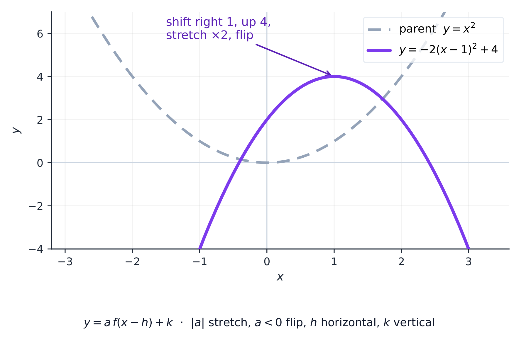
Transformations of graphs

A transformation 变换 builds a new function from an old one $f$:

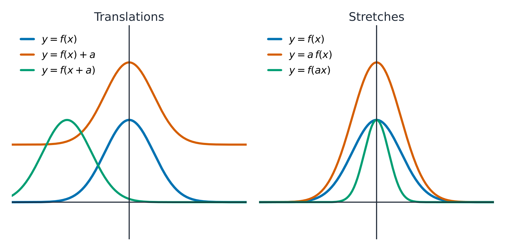
Adding to the output or input shifts the curve; a multiplier stretches it
  • Translations 平移 (shifts): $f(x)+k$ moves up/down; $f(x-h)$ moves right/left.
  • Dilations 伸缩 (stretches): $a\,f(x)$ stretches vertically by a factor of $|a|$; $f(bx)$ stretches horizontally by a factor of $\tfrac{1}{|b|}$ (so $f(2x)$ squeezes the graph to half its width).
  • Reflections 反射: $-f(x)$ flips over the $x$-axis; $f(-x)$ flips over the $y$-axis.

Combine additive shifts and multiplicative stretches to model shifted, scaled versions of a known shape.

Transforming the parent parabola: shift, stretch, and reflect
探索

探索平移、拉伸和翻转

选择平移、反射、旋转或放大并改变数量。观察哪些特征保持不变——变换移动整个图形而不改变其底层规则。

词汇 训练
English 中文 拼音
transformation/trænsfɔːˈmeɪʃn/ 变换 biàn huàn
Translations/trænˈsleɪʃnz/ 平移 píng yí
Dilations/daɪˈleɪʃnz/ 伸缩 shēn suō
Reflections/rɪˈflekʃnz/ 反射 fǎn shè
1.13

函数模型选择与假设阐述

教学大纲

学习目标 1.13.A: 识别合适的函数类型,为给定情境构建函数模型。

  • 1.13.A.1 线性函数用于对数据集或情境场景中表现出大致恒定变化率的数据集或方面进行建模。
  • 1.13.A.2 二次函数用于对数据集或情境场景中表现出大致线性变化率的数据集或方面进行建模,或对具有唯一最大值或最小值且大致对称的数据集进行建模。
  • 1.13.A.3 涉及面积或二维的几何场景通常可用二次函数建模。涉及体积或三维的几何场景通常可用三次函数建模。
  • 1.13.A.4 多项式函数用于对具有多个实数零点或多个极大值或极小值的数据集或情境场景进行建模。
  • 1.13.A.5 $n$ 次多项式函数用于对表现出大致恒定的非零 $n$ 阶差分的数据集或情境场景进行建模。
  • 1.13.A.6 次数不超过 $n$ 的多项式函数可用于对具有不同输入值的 $n + 1$ 个点构成的图形进行建模。
  • 1.13.A.7 分段定义函数由定义在不重叠定义域区间上的一组函数组成,适用于对在不同区间内表现出不同特征的数据集或情境场景进行建模。

学习目标 1.13.B: 描述与构建函数模型相关的假设和限制条件。

  • 1.13.B.1 模型可能包含关于模型中哪些因素保持一致的潜在假设。
  • 1.13.B.2 模型可能包含关于各变量如何共同变化的潜在假设。
  • 1.13.B.3 模型可能需要基于数学线索、情境线索或数据集中的极端值来限制定义域。
  • 1.13.B.4 模型可能需要基于数学线索、情境线索或数据集中的极端值来限制值域,例如对数值进行取整处理。

来源:College Board AP 课程与考试说明

English

Choosing a model 模型 means matching a function type to how a quantity changes. A linear model fits a constant rate of change; a quadratic fits a constant second difference; a polynomial fits data with several turns. In geometric situations the number of dimensions is a strong hint: quantities about area (two dimensions) are typically quadratic, and quantities about volume (three dimensions) are typically cubic – for example a box's volume as a function of a cut length. State the assumptions 假设 your model relies on (for example, that the pattern continues), because a model is only valid where those assumptions hold.

词汇 训练
English 中文 拼音
model/ˈmɒdl/ 模型 mó xíng
assumptions/əˈsʌmpʃnz/ 假设 jiǎ shè
1.14

函数模型的构建与应用

教学大纲

学习目标 1.14.A: 构建线性、二次、三次、四次、$n$ 次多项式或相关分段定义函数模型。

  • 1.14.A.1 可根据数学或实际情境中识别出的限制条件构建模型。
  • 1.14.A.2 可通过基本函数的变换,基于数据集或实际情境构建模型。
  • 1.14.A.3 可利用技术工具及回归分析(包括线性、二次、三次和四次回归)基于数据集构建模型。
  • 1.14.A.4 可通过组合建模技术构建分段定义函数模型。

学习目标 1.14.B: 基于实际情境构建有理函数模型。

  • 1.14.B.1 涉及成反比量的数据集及实际情境的某些方面,通常可用有理函数进行建模。例如,物体之间万有引力与电磁力的大小均与物体间距离的平方成反比。

学习目标 1.14.C: 应用函数模型回答关于数据集或实际情境的问题。

  • 1.14.C.1 可利用模型对建模后的数据集或实际情境得出结论,包括回答关键问题以及预测数值、变化率、平均变化率和变化率的变化。应根据给定上下文提取或推断适当的度量单位。

来源:College Board AP 课程与考试说明

English

To construct a model, use given features – points, intercepts, zeros with multiplicities, end behavior – to write the function, then use it to answer questions in context. Always check the answer against the domain that makes sense for the situation, and interpret outputs with their real-world units.

A piecewise-defined function 分段函数 uses different rules over non-overlapping intervals of the domain. To evaluate it, pick the branch whose interval contains the input. For example,

$$f(x)=\begin{cases} x^2, & x<0\\ 2x, & x\ge 0\end{cases}$$
gives $f(-3)=9$ from the first branch but $f(3)=6$ from the second – useful when behaviour changes at a threshold (a tiered price, a speed limit that changes).

词汇 训练
English 中文 拼音
piecewise-defined function/ˈpiːswaɪz dɪˈfaɪnd ˈfʌŋkʃn/ 分段函数 fēn duàn hán shù
1.14

考试技巧

English
  • Read a function through its rate of change: average rate = secant slope; a constant rate means linear, a linear-changing rate means quadratic.
  • Factor a polynomial to find zeros (x-intercepts) and their multiplicity; even multiplicity touches, odd crosses the axis.
  • End behaviour is set by the leading term; a rational function's asymptotes come from the degrees of top and bottom.
  • Build models from key features (points, zeros, end behaviour) and state your assumptions.
  • Describe transformations precisely: shift $f(x-h)+k$, stretch $af(bx)$, reflect $-f(x)$ / $f(-x)$.

该知识点的互动课程

逐步完成,配合即时检查练习。

历年真题

更多 AP 微积分预备 知识点

登录或创建账户

IGCSE, A-Level & AP