Edexcel IAL Physics Unit 1 (paper WPH11) is Mechanics and Materials 力学与材料: how things move, what forces do, how momentum and energy behave, and how solid and liquid materials respond to forces.
The paper is 1 hour 30 minutes, 80 marks, every question compulsory. It mixes multiple-choice, short answers, calculations and one or two extended-writing answers marked with an asterisk 星号 (*).
At least 32 of the 80 marks test Level-2 mathematics: reading graphs, rearranging equations, trigonometry 三角学 and areas.
A formula list is printed at the back of the paper. Learn what each symbol means and when each equation is allowed — the list gives formulas, not understanding.
Use $g = 9.81\ \text{m s}^{-2}$. The paper requires this value; using $g = 10$ can lose accuracy marks. Give final answers with a unit 单位 and a sensible number of significant figures 有效数字 (usually 2–3, matching the data).
A speedometer shows speed at one moment; a journey can still hide stops and bursts. This unit replaces one number with the full picture: graphs, vectors 矢量, forces 力, momentum 动量, energy 能量 and the strength of materials 材料.
displacement 位移 — straight-line change of position, with direction (a vector). distance 距离 — the total path length (a scalar 标量, no direction).
velocity 速度 — rate of change of displacement. speed 速率 — rate of change of distance.
acceleration 加速度 — rate of change of velocity: $a = \dfrac{\Delta v}{\Delta t}$, unit $\text{m s}^{-2}$.
Because displacement is the straight line from start to finish, a curved path always gives distance > magnitude of displacement — the examiner asks for exactly this comparison.
Reading motion graphs
On a displacement–time graph, the gradient 斜率 is the velocity. A curved line means changing velocity; take the gradient of a tangent 切线 at the point.
On a velocity–time graph, the gradient is the acceleration, and the area 面积 between the line and the time axis is the displacement. Area below the axis is negative displacement (motion backwards); distance adds the sizes of all the areas.
On an acceleration–time graph, the area under the line is the change in velocity.
Constant non-zero acceleration bends a displacement–time graph into a parabola 抛物线; a straight line on that graph means zero acceleration.
Worked example (June 2025 style). A velocity–time line rises straight from $1.8\ \text{m s}^{-1}$ at $t = 4\ \text{s}$ to $5.0\ \text{m s}^{-1}$ at $t = 16\ \text{s}$.
Known: two $(t, v)$ pairs on the straight part. Why: acceleration is the gradient of a velocity–time graph.
Check: the line rises gently, so a small acceleration is sensible.
The four suvat equations
For uniform acceleration 匀加速 (constant acceleration) in one dimension, with $s$ displacement, $u$ initial velocity, $v$ final velocity, $a$ acceleration, $t$ time:
$$v = u + at \qquad s = \frac{(u+v)t}{2} \qquad s = ut + \tfrac{1}{2}at^2 \qquad v^2 = u^2 + 2as$$
Choose the equation that contains your known quantities and the one you want — and nothing you do not know. No $t$? Use $v^2 = u^2 + 2as$. No $a$? Use $s = \tfrac{(u+v)}{2}t$.
These equations are valid only while the acceleration is constant. A curved velocity–time graph shows changing acceleration; a curved displacement–time graph can still represent constant acceleration.
Free fall is uniform acceleration with $a = g = 9.81\ \text{m s}^{-2}$ downwards (air resistance negligible 可忽略的).
Worked example (deduce-and-compare, June 2025 Q13). A basketball is thrown from $1.7\ \text{m}$ above the floor with initial vertical velocity $5.1\ \text{m s}^{-1}$ upwards, and enters the hoop moving downwards at $2.1\ \text{m s}^{-1}$. Is the hoop $3.0\ \text{m}$ above the floor?
Known: $u = +5.1\ \text{m s}^{-1}$, $v = -2.1\ \text{m s}^{-1}$ (downwards is negative), $a = -9.81\ \text{m s}^{-2}$. Wanted: the rise $\Delta s$. No time given, so use $v^2 = u^2 + 2a\Delta s$.
$$v^2 = u^2 + 2a\Delta s \quad\Rightarrow\quad \Delta s = \frac{v^2 - u^2}{2a}$$
Hoop height $= 1.7\ \text{m} + 1.1\ \text{m} = 2.8\ \text{m} \neq 3.0\ \text{m}$, so the hoop was not at the regulation height. A "deduce whether" question earns its last mark only when the comparison and conclusion are stated.
Core practical 1: measuring $g$
Drop an object and measure it: with a light gate 光电门 or video of known frame rate, get $s$ and $t$ (or velocities at two points) and use a suvat equation. Cleaner: plot $s$ against $t^2$ for $s = \tfrac{1}{2}gt^2$ — a straight line through the origin with gradient $g/2$. A straight line that misses the origin reveals a systematic offset 系统偏差, for example a fixed offset in the measured distance. A timing delay can also distort the relationship; automatic timing reduces reaction-time error. In a strobe photograph, the object moves during each flash. A shorter flash produces a sharper image and a smaller range of possible positions, reducing the uncertainty in the distance reading if the scale and image resolution are unchanged.
A vector has magnitude and direction (displacement, velocity, acceleration, force, momentum); a scalar has magnitude only (distance, speed, work, energy). Vector notation in the paper is an arrow above the symbol, $\vec{F}$.
Resolving and combining
Resolving splits one vector into two perpendicular 垂直的 components: the component of force $F$ at angle $\theta$ along a direction is $F\cos\theta$ if $\theta$ is measured from that direction, $F\sin\theta$ from the perpendicular. Choose by drawing the right triangle, not by habit.
Combining two perpendicular components rebuilds the vector: magnitude $R = \sqrt{F_x^2 + F_y^2}$, direction from $\tan\theta = F_y / F_x$.
Combine before squaring. The resultant of $500\ \text{N}$ and $200\ \text{N}$ at right angles is $\sqrt{500^2 + 200^2}\ \text{N}$, not $\sqrt{500^2} + \sqrt{200^2}$.
At any angle, add vectors by drawing a scale diagram 比例图 (a vector triangle, nose to tail) or by resolving each vector into components first. In equilibrium 平衡, the vector triangle closes: $\vec{W} + \vec{T_1} + \vec{T_2} = 0$.
Worked example. A box sits on a ramp at angle $\theta$ to the horizontal, weight $W$ acting vertically down.
Why: the sliding direction is along the ramp, so resolve $W$ into components along and perpendicular to the ramp.
At constant speed the resultant force is zero, so the friction $F = W\sin\theta$ exactly. ($W\cos\theta$ acts into the ramp and is balanced by the normal contact force.)
Projectile motion
A projectile 抛体 moving freely under gravity is two independent motions: horizontal velocity constant (no horizontal force), vertical velocity changing under $g$.
The time to fall depends only on the vertical motion. Two balls leaving a table at different speeds — or with different masses — land after the same time: mass and horizontal speed do not appear in $s = ut + \tfrac{1}{2}gt^2$.
Method: resolve the launch velocity into $u_h = u\cos\theta$ and $u_v = u\sin\theta$; run suvat separately for each direction; time links the two.
Worked example (January 2025 Q19). A projectile launches at $500\ \text{m s}^{-1}$, $22^\circ$ above the horizontal, from $2.0\ \text{km}$ above the sea. Show it passes over a ship $15\ \text{km}$ away after about $30\ \text{s}$.
Known: $u$, $\theta$, horizontal distance $s_h$. Horizontal motion has $a = 0$, so use $s_h = u_h t$.
Why a maximum range exists: raising the launch angle raises $u_v$ (more time in the air) but lowers $u_h$; range $= u_h \times t$ peaks between the two effects.
能够使用方程 ΣF = ma,并理解如何在质量 m 恒定的情况下应用此方程(牛顿第二运动定律),包括当 a = 0 时的牛顿第一运动定律:物体静止或以恒定速度运动;预期会使用术语“终端速度”。
能够使用重力场强度 g = F/m 和重量 W = mg 的方程。
了解并理解牛顿第三运动定律,并知道两个物体相互作用中成对力的性质。
แหล่งที่มา: หลักสูตร Cambridge International
English
A free-body diagram 受力图 shows only the forces acting on the chosen object — never forces the object applies to other things. On an extended body, the weight acts at the centre of gravity 重心.
Newton's first law 牛顿第一定律: zero resultant force means no change in motion — at rest or moving at constant velocity. Constant velocity is not "no forces"; it is balanced forces.
Newton's second law 牛顿第二定律: $\sum F = ma$. The resultant force causes the acceleration; list every force, choose a positive direction, then apply.
Newton's third law 牛顿第三定律: when body A exerts a force on body B, B exerts an equal, opposite force on A. The pair acts on different bodies, is the same type of force, and acts along the same line. A book's weight and the table's normal contact force are not a third-law pair: they act on the same body.
weight 重量$W = mg$; gravitational field strength 重力场强度$g = \dfrac{F}{m}$, so $g = 9.81\ \text{N kg}^{-1}$.
Terminal velocity 终端速度: as a falling object speeds up, drag 阻力 grows until drag (+ upthrust) equals weight; the resultant force is then zero and the velocity stops changing. "Terminal" describes the force balance, not a speed limit printed in nature.
Worked example (June 2025 Q11). A resultant force of $4800\ \text{N}$ accelerates a boat at $0.31\ \text{m s}^{-2}$. Find the boat's weight.
Known: $\sum F$, $a$. Why: $\sum F = ma$ links them to the mass; $W = mg$ links mass to weight.
$$\sum F = ma \quad\Rightarrow\quad m = \frac{\sum F}{a} = \frac{4800\ \text{N}}{0.31\ \text{m s}^{-2}} = 15\,500\ \text{kg}$$
momentum$p = mv$, a vector, unit $\text{kg m s}^{-1}$.
Conservation of linear momentum 动量守恒: when the resultant external force is zero (or its impulse during a short interaction is negligible), total momentum before an event equals total momentum after. Give velocities signs: choose one direction as positive and keep it.
Momentum conservation follows from Newton's second and third laws: the forces between the two bodies are equal and opposite, act for the same time, so the changes of momentum are equal and opposite.
Kinetic energy need not survive a collision; momentum always does (in an isolated system 孤立系统).
Worked example (June 2025 Q10). A train of mass $3m$ at speed $v$ meets a truck of mass $m$ at speed $2v$ the other way; they couple. Find the new speed.
Known: masses, velocities in opposite directions. Why: an isolated pair, so conserve momentum with signs. Take the train's direction as positive.
$$p_{\text{before}} = p_{\text{after}}$$
$$3m \times v + m \times (-2v) = (3m + m)\,V$$
$$mv = 4mV \quad\Rightarrow\quad V = \frac{v}{4}$$
Check: the momenta nearly cancel, so a small combined speed in the train's direction is sensible.
能够用力矩方程 moment of force = Fx 进行计算,其中 x 是力的作用线与旋转轴之间的垂直距离。
能够使用扩展物体的重心概念,并将力矩原理应用于处于平衡状态的扩展物体。
แหล่งที่มา: หลักสูตร Cambridge International
English
The moment of a force 力矩 about a pivot 支点 is $\text{moment} = Fx$, where $x$ is the perpendicular distance 垂直距离 from the pivot to the force's line of action. If the force meets the lever at angle $\theta$, use the perpendicular component $F\sin\theta$ or the perpendicular distance — never both.
Principle of moments 力矩原理: in equilibrium, total clockwise moment = total anticlockwise moment (resultant moment is zero).
Full equilibrium needs both: resultant force zero and resultant moment zero. A see-saw with equal children at equal distances has both; the same children at unequal distances still balance forces but not moments.
For a uniform 均匀的 beam, the weight acts at its centre.
Worked example (June 2025 Q19). A uniform rail, length $1.40\ \text{m}$, weight $95\ \text{N}$, lies at $42^\circ$ to the horizontal, pivoted at one end. A piston pushes with $160\ \text{N}$ at $18^\circ$ to the rail, $0.37\ \text{m}$ from the pivot. What perpendicular force $F$ at the handle end just lifts the rail?
Known: geometry, both forces, both angles. Why: just lifting means equilibrium at the pivot, so apply the principle of moments with perpendicular parts.
A vertical pull at the handle instead: its perpendicular distance to the pivot is shorter than the rail's length, so a larger force would be needed for the same moment.
work 功$\Delta W = F\Delta s$ when the force acts along the motion; if the force is at angle $\theta$ to the motion, only the component along the motion works: $\Delta W = F\Delta s\cos\theta$.
kinetic energy 动能$E_k = \tfrac{1}{2}mv^2$ — doubling speed quadruples the energy.
gravitational potential energy 重力势能$\Delta E_{\text{grav}} = mg\Delta h$ near the Earth's surface.
Conservation of energy 能量守恒: energy is transferred or transformed, never created or destroyed. In a fall with drag, $\Delta E_{\text{grav}}$ becomes $E_k$plus work done against air resistance; at terminal velocity $E_k$ is constant, so all of the $\Delta E_{\text{grav}}$ goes to work against drag.
power 功率$P = \dfrac{E}{t} = \dfrac{W}{t}$ — energy transferred per unit time.
efficiency 效率$= \dfrac{\text{useful energy output}}{\text{total energy input}} = \dfrac{\text{useful power output}}{\text{total power input}}$.
Worked example (June 2025 Q14). An electric car of $1800\ \text{kg}$ at $14\ \text{m s}^{-1}$ brakes to rest on a hill, gaining $0.76\ \text{m}$ of height; the battery gains $45\ \text{kJ}$. Find the efficiency of the braking.
Known: $m$, $v$, $\Delta h$, battery gain. Why: the total input is the energy the brakes remove — kinetic energy lost minus the gravitational energy the car keeps by ending higher.
a) สามารถใช้สมการสำหรับแรงต้านความหนืด (กฎของสโตกส์) F = 6πηrv; b) เข้าใจว่าสมการนี้ใช้ได้เฉพาะกับวัตถุทรงกลมขนาดเล็กที่เคลื่อนที่ด้วยความเร็วต่ำและมีการไหลแบบลามินาร์ (หรือไม่มีกระแสไหลแบบวุ่นวาย) และความหนืดขึ้นอยู่กับอุณหภูมิ
density 密度$\rho = \dfrac{m}{V}$. For a sphere, $V = \tfrac{4}{3}\pi r^3$.
upthrust 浮力 = weight of the fluid displaced 排开的流体 — the displaced weight, not its volume or its mass.
Stokes' law 斯托克斯定律: viscous drag on a small sphere at low speed in laminar flow 层流 is $F = 6\pi\eta rv$, with $\eta$ the viscosity 黏度, $r$ the radius, $v$ the speed. It is valid only for small spheres moving slowly without turbulence 湍流, and $\eta$ falls as the liquid warms in this experiment; gases do not generally follow this trend.
Core practical 2: viscosity by the falling-ball method
Drop a ball-bearing into a measuring cylinder of the liquid. Wait until it falls at terminal velocity, then time it over a marked distance. At terminal velocity, the forces balance: weight = upthrust + drag, so
You need the ball's radius and mass (or its density), the oil's density, the fall distance and the time. Warm oil is less viscous, so the ball falls faster and the measured time is shorter.
a) สามารถวาดและตีความกราฟแรง–ระยะยืดและกราฟแรง–ระยะอัด; b) เข้าใจศัพท์จำกัดสัดส่วน, ขอบเขตยืดหยุ่น, จุดหย่อนตัว, การเปลี่ยนรูปยืดหยุ่น และการเปลี่ยนรูปพลาสติก และสามารถนำไปใช้กับกราฟเหล่านี้ได้
สามารถคำนวณพลังงานความเครียดยืดหยุ่น Eel ในตัวอย่างวัสดุที่เปลี่ยนรูป โดยใช้สมการ ΔEel = ½FΔx, และจากพื้นที่ใต้กราฟแรง–ระยะยืด; คาดหวังให้สามารถประมาณค่าพื้นที่และดังนั้นพลังงานเปลี่ยนแปลงสำหรับกราฟแรง–ระยะยืดทั้งเชิงเส้นและไม่เชิงเส้น
แหล่งที่มา: หลักสูตร Cambridge International
English
Hooke's law 胡克定律: $\Delta F = k\,\Delta x$ while the material behaves proportionally; $k$ is the stiffness 刚度 (spring constant 弹簧常数), the gradient of the force–extension graph.
stress 应力$\sigma = \dfrac{F}{A}$ (unit Pa), strain 应变$\varepsilon = \dfrac{\Delta x}{x}$ (no unit), Young modulus 杨氏模量$E = \dfrac{\sigma}{\varepsilon}$. Stress and strain describe the material; force and extension describe the sample.
On a force–extension or stress–strain graph: the straight part ends at the limit of proportionality 比例极限; beyond the elastic limit 弹性极限 the sample no longer returns to its original length (elastic deformation 弹性形变 = it does return; plastic deformation 塑性形变 = it stays stretched); a material with a distinct yield point can stretch substantially with little increase in force at yield; other ductile materials yield gradually. The yield point 屈服点 marks the onset of substantial plastic flow; the breaking stress 断裂应力 is the stress at fracture.
elastic strain energy 弹性应变能: $\Delta E_{\text{el}} = \tfrac{1}{2}F\Delta x$ for a linear spring — the area under the force–extension graph. For a non-linear graph, estimate the area by squares. The area under a loading stress–strain graph is the work done per unit volume 单位体积, because $\dfrac{F}{A} \times \dfrac{\Delta x}{x} = \dfrac{F\Delta x}{V}$. In the elastic region this is stored recoverably as elastic strain energy; work beyond the elastic limit is not all recoverable.
Worked example (June 2025 Q17b). A violin string of original length $0.750\ \text{m}$ and radius $0.85 \times 10^{-3}\ \text{m}$ stretches to $0.752\ \text{m}$ under $36\ \text{N}$. Find the Young modulus.
Known: $F$, $x$, $\Delta x$, $r$. Why: $E = \sigma/\varepsilon$ needs stress and strain; stress needs the cross-sectional area.
Check: a metal-wire modulus is $10^{9}$–$10^{12}\ \text{Pa}$; $6\ \text{GPa}$ sits in range.
Core practical 3: the Young modulus of a wire
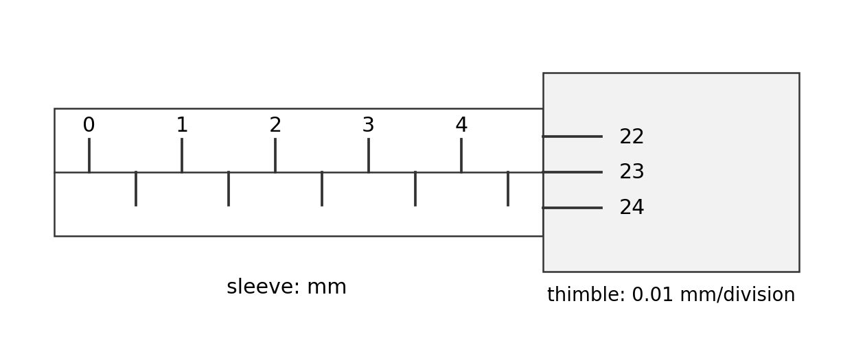
Hang known weights on a long wire and measure the extension with a marker against a scale; keep the wire long and the extensions small for precision, add loads in steps within the proportional region, and measure the diameter in several places with a micrometer 千分尺. Then $E$ comes from the gradient of the stress–strain line, or from $\sigma/\varepsilon$ point by point within the proportional region.
limit of proportionality/ˈlɪmɪt ɒv prəˌpɔːʃəˈnælɪti/
ขีดจำกัดความแปรผัน
elastic limit/ɪˈlæstɪk ˈlɪmɪt/
ขีดจำกัดยืดหยุ่น
elastic deformation/ɪˈlæstɪk ˌdiːfɔːˈmeɪʃn/
การเปลี่ยนรูปแบบยืดหยุ่น
plastic deformation/ˈplæstɪk ˌdiːfɔːˈmeɪʃn/
การเปลี่ยนรูปแบบพลาสติก
yield point/jiːld pɔɪnt/
จุดหย่อน
breaking stress/ˈbreɪkɪŋ stres/
ความเครียดที่หัก
elastic strain energy/ɪˈlæstɪk streɪn ˈenədʒi/
พลังงานความยืดหยุ่น
per unit volume/pɜː ˈjuːnɪt ˈvɒljuːm/
ต่อหน่วยปริมาตร
micrometer/maɪˈkrɒmɪtə/
ไมโครมิเตอร์สกรู
1.8
Exam craft for WPH11
English
Show every step. "Use of $F = ma$" earns a mark before any number appears — write the equation in symbols, then substitute.
Units and $g$. A missing unit usually loses the final mark; $g = 10\ \text{m s}^{-2}$ can lose accuracy marks; "show that" questions need one more significant figure than the target value.
Command words:state = a short precise answer; calculate/determine = numbers with working and a unit; deduce = working plus a compared conclusion; explain = linked physics reasons; describe = what happens, in order.
The asterisk (*) answer is marked for linked, logical reasoning as well as content: order the points, then link them.
The formula list is at the back — know where, so you never memorise what you can look up in two seconds.
1.8
ตรวจสอบตัวเอง
English
On a velocity–time graph, what do the gradient and the area give? — acceleration; displacement.
Which suvat equation finds a height from two velocities without time? — $v^2 = u^2 + 2as$.
A projectile's horizontal acceleration in free flight? — zero (only gravity acts, vertically).
A book rests on a table: are its weight and the table's normal force a Newton's-third-law pair? — No: they act on the same body.
Two trolleys collide and stick. Which quantity is always conserved? — total momentum (kinetic energy need not be).
A force at an angle to a lever: which distance goes into the moment? — the perpendicular distance from the pivot to the line of action.
A car brakes uphill: what is the input energy for the efficiency? — the kinetic energy lost minus the gravitational energy gained.
Upthrust equals the weight of what? — the fluid displaced.
Stokes' law needs which three conditions? — small sphere, low speed, laminar flow (and $\eta$ is temperature-dependent).
On a stress–strain graph, what is the gradient of the straight part, and what is the area beneath it? — the Young modulus; the elastic strain energy per unit volume.
Your phone receives waves and uses electrical energy. These seem different, but both depend on energy transfer. Waves 波 carry energy without carrying matter along with them. A circuit transfers energy through moving charge.
This reference covers WPH12 Waves and Electricity, specification statements 33–80. The paper lasts 90 minutes and carries 80 marks. Use the formula list to support your reasoning. Explain why an equation fits the situation, show conversions, and finish comparisons with a conclusion.
Wave quantities and graphs
A vibrating source repeats its motion. The amplitude 振幅 is the greatest displacement from equilibrium. Equilibrium 平衡位置 means the resting position. The period 周期$T$ is the time for one complete vibration. The frequency 频率$f$ is the number of complete vibrations each second; its unit is hertz, Hz.
$$f = \frac{1}{T} \qquad v = f\lambda$$
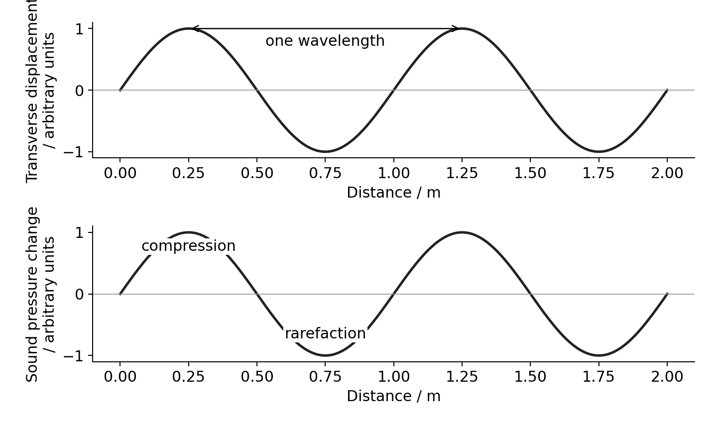
The wavelength 波长$\lambda$ is the distance between nearest points vibrating in phase. The wave speed 波速$v$ is the speed at which a fixed phase, such as a crest, travels. It is not the speed of a vibrating particle.
A transverse wave 横波 has vibrations perpendicular to its direction of travel. A rope moves up and down while its disturbance travels along the rope.
A longitudinal wave 纵波 has vibrations parallel to its direction of travel. Sound has compressions 密部, where pressure and density are higher, and rarefactions 疏部, where they are lower.
Air molecules move back and forth about their resting positions. They do not travel from the speaker to your ear with the sound.
Distance graphs show a whole wave at one instant.
Read the horizontal axis first
A displacement–distance graph is a snapshot. The separation of neighbouring crests gives $\lambda$. A displacement–time graph follows one particle. The separation of neighbouring peaks gives $T$. The same curve shape can represent either graph, but the quantities are different.
For a longitudinal wave, a pressure–distance graph shows compressions at pressure maxima. A molecular displacement–distance graph shows displacement along the direction of travel. Maximum compression occurs where displacement changes most rapidly towards the neighbouring molecules. Pressure maximum and displacement maximum are not at the same place; their patterns are one-quarter wavelength apart in a sinusoidal travelling sound wave.
Worked example. A microphone records 12 complete cycles in $0.030\ \text{s}$. Sound travels at $340\ \text{m s}^{-1}$. Find its frequency and wavelength.
Known: cycle count, total time and speed. Frequency counts cycles per second; the wave equation then links speed to wavelength.
Check: one cycle takes $T=1/f=0.0025\ \text{s}$. Twelve cycles take the stated $0.030\ \text{s}$.
Superposition and standing waves
A wavefront 波阵面 joins points at the same phase. Phase 相位 describes the stage of a vibration cycle. One complete cycle corresponds to $360^\circ$ or $2\pi$ radians.
Superposition 叠加 means adding the displacements of overlapping waves at each point. Interference 干涉 is the resulting reinforcement or cancellation. Coherent sources 相干波源 have the same frequency and a constant phase difference. Their phase difference need not be zero.
For waves of the same wavelength, the phase difference caused by a path difference 路程差$\Delta x$ is:
For sources initially in phase, path differences $0,\lambda,2\lambda,\ldots$ give constructive interference. Half-integer wavelength differences give destructive interference. Complete cancellation also needs equal amplitudes. If sources start with a phase difference, include it too.
Worked example. Two in-phase speakers produce wavelength $0.80\ \text{m}$. Their paths to a microphone differ by $1.20\ \text{m}$.
Known: path difference and wavelength. Convert path difference into cycles, then phase.
$540^\circ$ is equivalent to $180^\circ$. The waves arrive in opposite phase and interfere destructively. The sound need not become silent if the arriving amplitudes differ.
How a standing wave forms
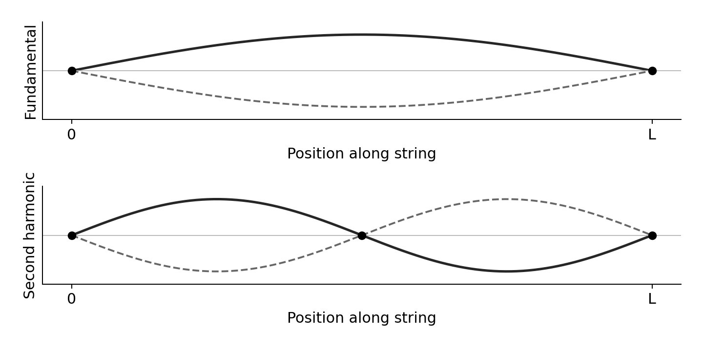
A standing wave 驻波 forms when two waves of the same frequency and similar amplitude travel in opposite directions and superpose. Reflection at a fixed string end supplies the returning wave.
A node 波节 always has zero displacement. An antinode 波腹 has the largest vibration amplitude.
Adjacent nodes are $\lambda/2$ apart. A node and its nearest antinode are $\lambda/4$ apart.
Points between the same pair of nodes vibrate in phase. Points in neighbouring sections vibrate in opposite phase.
All points have the same frequency, except that a node does not vibrate. Amplitude depends on position.
An ideal standing wave has no net energy transfer along it. A travelling wave carries energy along its direction of travel.
The end nodes remain still; the curve changes between the solid and dashed shapes.
For a string fixed at both ends, length $L$ contains a whole number $k$ of half-wavelengths:
$$L = \frac{k\lambda}{2} \qquad v = \sqrt{\frac{T}{\mu}} \qquad f = \frac{k}{2L}\sqrt{\frac{T}{\mu}}$$
Here $T$ is tension 张力, not period; $\mu$ is mass per unit length 线密度 in $\text{kg m}^{-1}$. The fundamental has $k=1$. At fixed mode, frequency increases with $\sqrt{T}$, decreases with $L$, and decreases with $\sqrt{\mu}$.
Worked example. A $0.60\ \text{m}$ string has $\mu=1.5\times10^{-3}\ \text{kg m}^{-1}$ and tension $24\ \text{N}$. Find its fundamental frequency.
Known: length, tension and linear density. The fundamental fits half a wavelength between the fixed ends.
Doubling tension multiplies frequency by $\sqrt{2}$, rather than by two.
Standing sound in a closed tube
In the simplest standing sound wave in a tube closed at one end, the closed end is a molecular displacement node. The open end is approximately a displacement antinode. This fits one-quarter wavelength into the effective tube length, so $L_{effective}=\lambda/4$. The pressure pattern is reversed: the closed end is a pressure antinode. Do not call a pressure node a displacement node. Real tubes have a small open-end correction; use an effective length if the question supplies it.
Worked example. A closed tube has effective length $0.20\ \text{m}$ and fundamental frequency $425\ \text{Hz}$. The end conditions give $\lambda=4L=0.80\ \text{m}$; then $v=f\lambda=425\times0.80=340\ \text{m s}^{-1}$. A string fixed at both ends instead fits half a wavelength in its fundamental. Choose from the end conditions, not from the word “standing”.
Core practical 4: speed of sound
Use a signal generator, speaker, movable microphone and two-beam oscilloscope 双踪示波器. Connect one oscilloscope channel to the generator reference signal and the other to the microphone output. Both traces have the same frequency.
Keep frequency constant. Move the microphone along a measured line away from the speaker. Find a position where the traces are in phase.
Move to another in-phase position. Consecutive in-phase positions are one wavelength apart. Measure across several wavelengths and divide by their number.
Read the period from the time-base scale: count horizontal divisions across several cycles, then divide. Find $f=1/T$ and use $v=f\lambda$.
Repeat positions and frequencies. Keep the microphone on the speaker axis. Reduce reflected sound by working away from walls. Measure position from a fixed microphone reference point.
Measuring several wavelengths reduces the percentage uncertainty in the distance. Measuring several periods does the same for time. A resonance-tube experiment can also measure sound speed, but it does not replace this specified practical.
Core practical 5: vibrating string
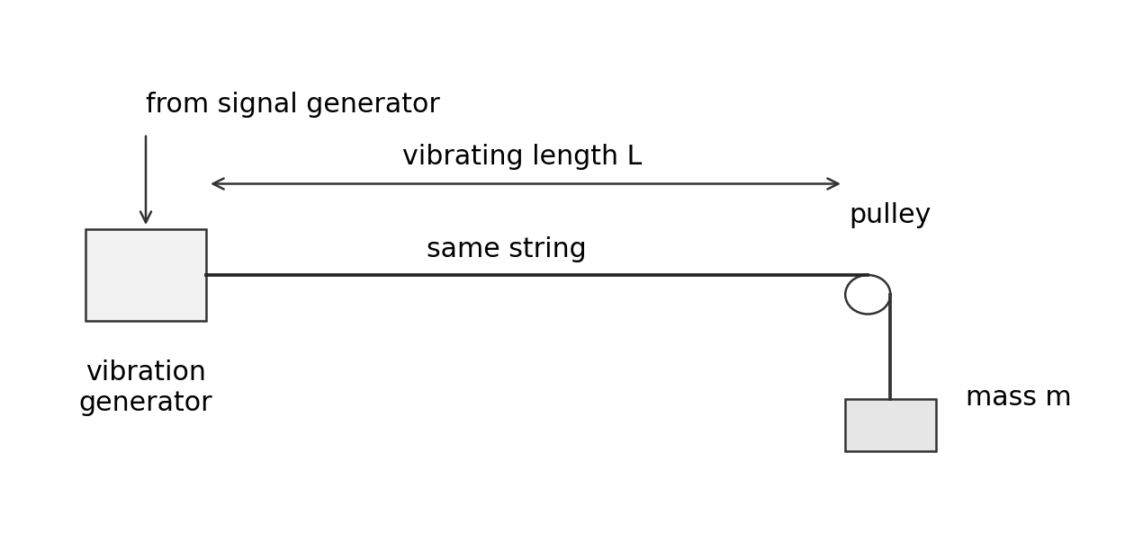
Use a vibration generator driven by a signal generator. Run the string over a pulley to a hanging mass. The tension is about $mg$ when pulley friction is small. Increase frequency until a clear standing-wave pattern forms.
Investigate tension: keep $L$, $\mu$ and mode fixed. Vary hanging mass. Plot $f^2$ against $T$; the gradient for the fundamental is $1/(4L^2\mu)$.
Investigate length: keep tension, string type and mode fixed. Plot $f$ against $1/L$.
Investigate linear density: measure string mass and length, $\mu=m/l$. Use different strings with fixed tension, vibrating length and mode. Plot $f^2$ against $1/\mu$.
Measure length between the end nodes. Find the resonance from both higher and lower frequencies and repeat. Secure the stand and keep clear of falling masses.
Intensity, refraction and polarisation
Intensity 强度 is power per unit area perpendicular to the energy flow:
$$I = \frac{P}{A}$$
Its unit is $\text{W m}^{-2}$. For a receiver, incident power is $P=IA$. Useful output is smaller if efficiency is below 100%. Convert area carefully: $1\ \text{cm}^2=10^{-4}\ \text{m}^2$.
Worked example. Radiation intensity is $800\ \text{W m}^{-2}$ over a $25\ \text{cm}^2$ solar cell. Efficiency is 20%. Can it supply $0.50\ \text{W}$?
Known: intensity, area, efficiency. First find incident power, then useful power.
$0.40\ \text{W}<0.50\ \text{W}$, so it cannot supply the required useful power.
Refraction and total internal reflection
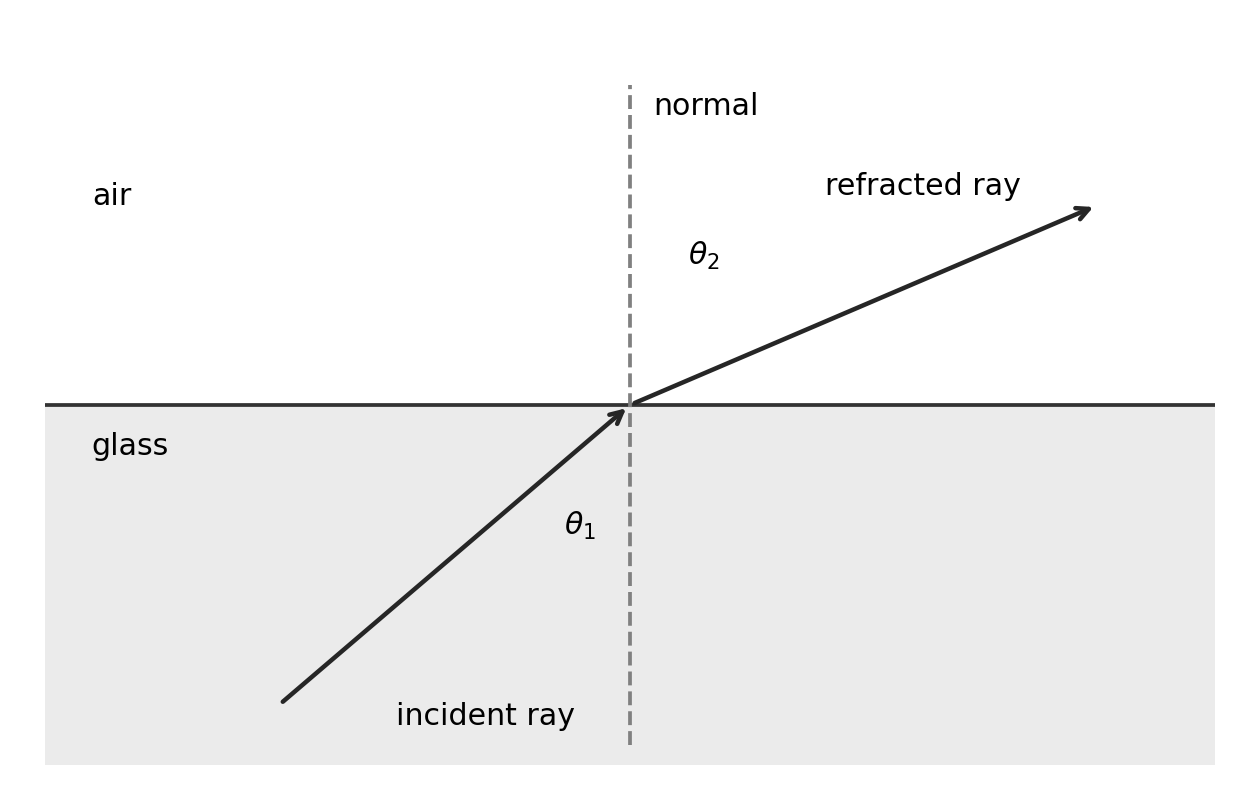
Refraction 折射 is a change in wave direction when speed changes at an interface. A ray entering along the normal changes speed without changing direction. The normal 法线 is perpendicular to the boundary. Measure all ray angles from it.
The refractive index 折射率$n$ compares vacuum light speed $c$ with speed in the material. Frequency stays constant across the boundary, so wavelength changes with speed. Entering higher $n$ bends the ray towards the normal; entering lower $n$ bends it away.
The ray bends away from the normal when it enters the lower-index medium.
Total internal reflection 全反射 requires travel from higher to lower refractive index and incidence greater than the critical angle 临界角$C$.
$$\sin C = \frac{n_2}{n_1} \qquad \text{for material to air: }\sin C = \frac{1}{n}$$
At $C$ the refracted angle is $90^\circ$; call incidence greater than $C$ total internal reflection. Below $C$, some energy is normally reflected and some transmitted. An optical fibre uses a higher-index core and lower-index cladding. Raising the cladding index raises the critical angle and can stop a previously reflected ray being trapped.
Worked example. Light travels from glass of index 1.50 into air. Does an incidence angle of $45^\circ$ produce total internal reflection?
Known: the two indices and incidence angle. Find the boundary angle before comparing.
The light travels towards lower index and $45^\circ>41.8^\circ$. Both conditions hold, so total internal reflection occurs.
Measuring refractive index
Place a rectangular transparent block on paper and trace its outline. Use a narrow ray-box beam. Mark two points on the incident ray and two on the emerging ray. Remove the block and join the boundary points to reconstruct the ray inside. Draw the normal at entry and measure incidence $i$ and refraction $r$ with a protractor.
Repeat for several incidence angles, keeping the same material and light colour. Plot $\sin i$ vertically against $\sin r$ horizontally. For air into the block, the gradient is the block's refractive index relative to air. Use a large triangle on a best-fit line. Narrow beams and widely separated ray marks reduce direction uncertainty. Very small angles give large percentage angle uncertainties.
Plane polarisation
Plane polarisation 平面偏振 restricts transverse vibrations to one plane containing the propagation direction. Unpolarised light has vibrations in many planes. A polariser transmits one vibration direction. Rotate a second polariser: parallel transmission directions give maximum brightness; perpendicular directions ideally give darkness. The ray still travels forward; its vibration direction changes selection.
Longitudinal waves cannot be plane polarised because their vibration is already along propagation. Polarisation is therefore evidence that light is transverse.
Diffraction and pulse-echo
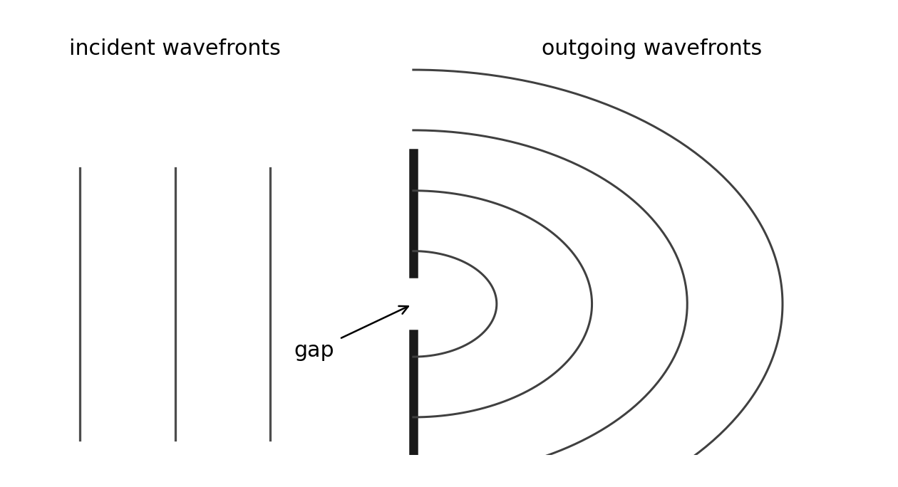
Diffraction 衍射 is the spreading of waves at a gap or edge. Spreading is greater when the gap width is comparable to the wavelength. A wide gap still diffracts at its edges, but the central wave spreads less.
In Huygens' construction 惠更斯作图法, each point on a wavefront acts as a source of secondary wavelets. Draw wavelets of equal radius after the same time. Their forward common tangent gives the new wavefront. At a narrow gap only a small part of the original front supplies wavelets, so the emerging fronts spread widely. This explains spreading without inventing a change of frequency at the slit.
The gap limits which points supply the outgoing wavelets.
Gratings and core practical 6
A diffraction grating 衍射光栅 contains many equally spaced slits. Bright maxima occur when contributions from neighbouring slits arrive in phase:
$$k\lambda = d\sin\theta$$
Here $k$ is the integer order 级次, $d$ is slit spacing, and $\theta$ is measured from the straight-through direction. The equation assumes normal incidence. If the grating has $N$ lines per metre, $d=1/N$. Do not confuse grating order with refractive index; printed papers may use $n$ for either.
Worked example. A grating has 600 lines per millimetre. First-order light appears at $18.0^\circ$. Find its wavelength.
Known: line density and first-order angle. Convert line density before taking its reciprocal.
This is $515\ \text{nm}$. Check each proposed higher order using $k\lambda/d\leq1$.
For CP6, aim a low-power laser normally at a grating and place a screen perpendicular to the central beam. Measure screen distance $D$ and displacement $x$ from the central spot to an order. Use $\tan\theta=x/D$, then the grating equation. Average corresponding left/right displacements, repeat distances, and use higher visible orders where measurement is clear. Measure from the grating to the screen, not from the laser casing. Do not substitute $\sin\theta=x/D$ unless a justified small-angle approximation is acceptable. Never look into the beam; keep it below eye level and stop stray beams.
Electrons also show wave behaviour
An electron beam passing through a thin crystal produces a diffraction pattern. Regular atom spacing provides the diffracting structure. Changing electron momentum changes the pattern spacing. This is evidence of wave behaviour; particles travelling along simple straight paths alone cannot explain the diffraction maxima.
The de Broglie wavelength 德布罗意波长 is:
$$\lambda = \frac{h}{p}$$
For a non-relativistic electron, $p=mv$. If it gains kinetic energy by crossing a potential difference, $E_k=eV$ and $p=\sqrt{2mE_k}$. Use these links only when the question gives or requires that energy relation.
Worked example. An electron has momentum $2.0\times10^{-24}\ \text{kg m s}^{-1}$. With $h=6.63\times10^{-34}\ \text{J s}$:
Increasing momentum reduces wavelength. Electrons have both particle and wave properties; diffraction does not mean that an electron becomes a sound wave.
Reflection, transmission and echoes
At an interface, part of a wave's energy may be transmitted 透射 and part reflected. A reflected pulse can locate a boundary. In pulse-echo 脉冲回波, measured delay includes the outward and return journeys:
$$2s = vt \quad\Rightarrow\quad s = \frac{vt}{2}$$
Worked example. Ultrasound travels in metal at $5900\ \text{m s}^{-1}$. An echo returns after $12\ \mu\text{s}$.
The boundary is $35\ \text{mm}$ away, not $71\ \text{mm}$. A nearby echo may overlap the transmitted pulse. Shorter pulse duration reduces this blind region and separates close echoes. Shorter wavelength helps detect or distinguish smaller features. These are related limits, but pulse duration and wavelength are not the same quantity. Use the speed in the actual material, not automatically the speed in air.
Photons and the photoelectric effect
Wave ideas explain interference, diffraction and polarisation. They did not explain all observations of energy transfer. Photons 光子 describe discrete packets of electromagnetic energy:
$$E = hf = \frac{hc}{\lambda}$$
Historically, interference and diffraction supported wave models of light. Quantum ideas developed to explain observations including the photoelectric effect and atomic spectra. Modern physics uses both wave and photon descriptions according to the measurement. A successful new model must explain evidence that the older model explains too.
One photon and one electron
In the photoelectric effect 光电效应, a surface electron absorbs a photon and may escape. The work function 逸出功$\phi$ is the minimum energy needed to remove an electron from the surface. The threshold frequency 极限频率 is $f_0=\phi/h$.
Below threshold, increasing intensity does not cause emission in the usual single-photon model.
Above threshold, higher frequency raises maximum kinetic energy. A graph of $E_{k,\max}$ against $f$ has gradient $h$, frequency intercept $f_0$ and extrapolated energy intercept $-\phi$.
At fixed frequency above threshold, higher intensity supplies more photons per second. More electrons can be emitted per second, so the saturation photocurrent rises. Their maximum kinetic energy does not rise.
Emission starts without the energy-building delay predicted by a simple continuous-wave energy model, even at low intensity above threshold.
Electrons escape with a range of kinetic energies. Some lose more energy within the material. The equation describes the largest energy, not every electron's energy.
The electronvolt 电子伏特 is an energy unit: $1\ \text{eV}=1.60\times10^{-19}\ \text{J}$. It is not a unit of potential difference. A stopping potential $V_s$ just prevents even the fastest photoelectrons reaching the collector, so $eV_s=E_{k,\max}$.
Worked example. Light of frequency $8.0\times10^{14}\ \text{Hz}$ reaches a surface with work function $2.0\ \text{eV}$.
Known: photon frequency and work function. Convert the work function into joules before subtracting.
The positive kinetic energy confirms that this frequency is above threshold. A negative subtraction would mean no emission, not negative kinetic energy.
Atomic line spectra
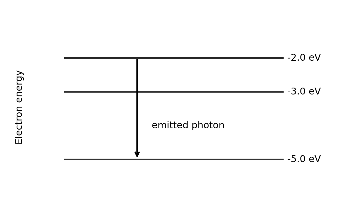
Atoms have discrete energy levels 分立能级. An electron moving down between two allowed levels emits a photon. Moving up requires absorption of the matching energy:
$$|\Delta E| = hf = \frac{hc}{\lambda}$$
A line spectrum has particular frequencies because only certain level differences are allowed. The largest downward energy difference gives the highest frequency and shortest wavelength. Count possible transitions by checking level pairs and which upper levels are populated; do not automatically count the number of levels as the number of lines.
The photon energy equals the difference between the two levels.
Worked example. An electron drops from $-2.0\ \text{eV}$ to $-5.0\ \text{eV}$.
Photon absorption in a material does not always eject an electron from its surface. Excitation followed by emission, for example in a light-activated material, is not automatically the photoelectric effect.
Current, resistance and circuits
Current 电流 is the rate of charge flow. Conventional current follows the direction positive charges would move. In a metal, electrons drift in the opposite direction.
$$I = \frac{\Delta Q}{\Delta t} \qquad V = \frac{W}{Q} \qquad R = \frac{V}{I}$$
One ampere is one coulomb per second. Potential difference 电势差$V$ is energy transferred per unit charge between two points. Resistance $R$ is defined by the ratio $V/I$ at an operating point. Ohm's law 欧姆定律 is the extra condition $I\propto V$ when temperature and other physical conditions stay constant. Not every resistor or component obeys it.
Worked example. A current of $0.40\ \text{A}$ flows for $30\ \text{s}$. Find the number of electrons passing a point.
$$Q = It = 0.40\ \text{A}\times30\ \text{s} = 12\ \text{C}$$
Charge conservation 电荷守恒 means charge does not build up at a steady-current junction. Total current entering equals total current leaving. Current is not used up by a resistor.
Energy conservation 能量守恒 means the total energy supplied per coulomb around a complete loop equals the energy transferred per coulomb. The sum of voltage rises equals the sum of voltage drops.
For series resistors, the same current passes through each and their potential differences add:
A parallel combination has smaller resistance than its smallest branch resistance. A voltmeter connects in parallel across a component; an ideal voltmeter has infinite resistance. An ammeter connects in series; an ideal ammeter has zero resistance.
Worked example. A $6.0\ \Omega$ resistor is parallel to $3.0\ \Omega$. The combination is in series with $4.0\ \Omega$ across $12\ \text{V}$.
Known: circuit arrangement. Reduce the parallel section first, then apply the series rule.
Check: branch currents add to $2.0\ \text{A}$. The remaining series resistor has an $8.0\ \text{V}$ drop.
Power and component graphs
Electrical power 电功率 is energy transferred each second. Substituting $V=IR$ into $P=VI$ gives the other forms:
$$P = VI = I^2R = \frac{V^2}{R} \qquad W = Pt = VIt$$
Use voltage across, and current through, the same component. The resistance forms apply to its operating-point resistance; do not assume a heating lamp has constant resistance.
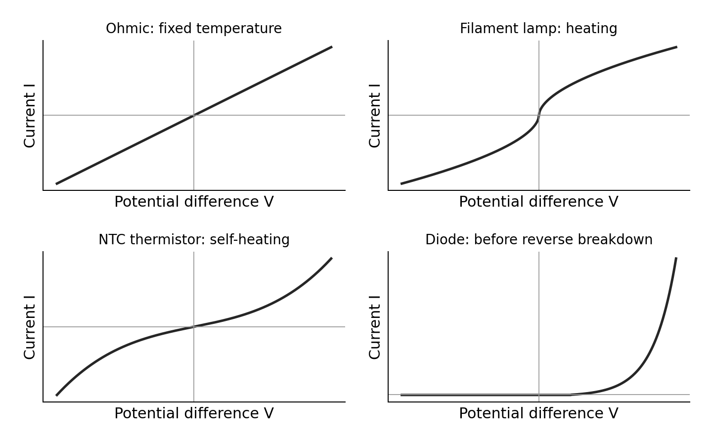
Axes and temperature conditions matter when interpreting these schematic curves.
Ohmic conductor at constant temperature: straight line through the origin. On an $I$-vertical, $V$-horizontal graph its gradient is $1/R$.
Filament lamp: as voltage magnitude rises, heating increases resistance. The $I$–$V$ curve becomes less steep.
NTC thermistor: heating lowers resistance. If current heats it sufficiently, the curve becomes steeper. At a controlled fixed temperature its behaviour over a suitable range can be approximately ohmic. Do not claim every thermistor curve must bend under every measurement condition.
Diode: very small reverse current before breakdown; forward current rises rapidly after a characteristic knee. It conducts mainly in one direction. A real diode does not have one constant resistance.
For a curved graph, $R=V/I$ uses a line from the origin to the operating point. The tangent gradient is not generally $1/R$.
Resistivity and core practical 7
Resistivity 电阻率$\rho$ is a material property at a stated temperature:
$$R = \frac{\rho l}{A} \qquad A = \frac{\pi d^2}{4}$$
Lengthening a uniform wire increases resistance. Increasing cross-sectional area decreases it. Doubling diameter gives four times the area and one-quarter the resistance, if material, length and temperature stay unchanged.
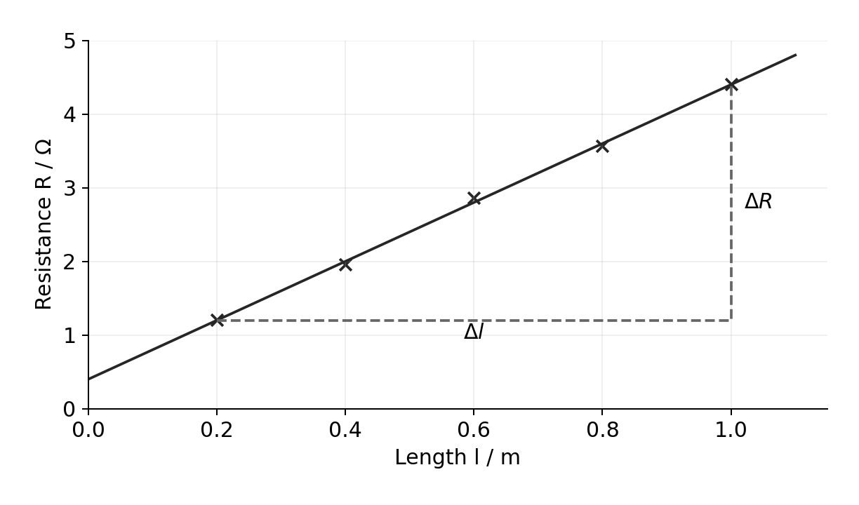
For CP7, connect a uniform wire, ammeter, power supply, switch and current-limiting resistor in series. Connect a voltmeter across the measured wire length. Measure several lengths and find $R=V/I$ for each. Plot $R$ against $l$: gradient $=\rho/A$, so $\rho=A\times\text{gradient}$.
Measure diameter with a micrometer at several positions and orientations; check its zero. Measure length between the actual electrical contacts. Use a small current and switch off between readings to limit heating. Keep contacts secure. A non-zero intercept may indicate contact or lead resistance. Repeating readings reduces scatter but does not remove a diameter zero error. Because area depends on $d^2$, a small percentage diameter uncertainty contributes about twice that percentage to area uncertainty.
Worked example. A wire diameter is $0.40\ \text{mm}$. An $R$–$l$ graph has gradient $3.5\ \Omega\,\text{m}^{-1}$.
The drift velocity 漂移速度$v$ is the small mean directed velocity of charge carriers, not their random thermal speed:
$$I = nqvA$$
Here $n$ is the number of mobile carriers per unit volume, $q$ is charge magnitude per carrier, and $A$ is cross-sectional area. A larger carrier density allows the same current with a smaller drift speed. In series wires the current is the same; changing $n$ or $A$ changes $v$.
Materials have different resistivities because their carrier densities and the ease of carrier motion differ. More scattering reduces drift speed for the same applied potential gradient. Carrier density alone does not explain every difference between materials.
Potential dividers, sensors and cells
Along a uniform wire carrying steady current at constant temperature, resistance grows in proportion to distance. The potential drop therefore grows in proportion to distance too. A potential–distance graph is straight. This assumes uniform material and area; a tapered or unevenly heated wire need not give a straight line.
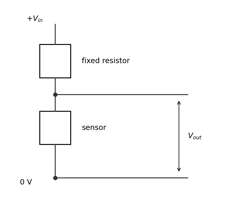
A potential divider 分压器 uses series resistances to share a supply voltage:
The expression assumes the output is unloaded, or the attached load draws negligible current. If a load draws significant current, combine it in parallel with the output resistor first. Always identify which resistor the voltmeter spans.
Swapping the sensor and fixed resistor reverses the direction of the output change.
Worked example. A $6.0\ \text{V}$ supply feeds a $2.0\ \text{k}\Omega$ fixed resistor above an LDR. Find the output across the LDR when its resistance changes from $4.0$ to $1.0\ \text{k}\Omega$.
The output across this LDR falls when illumination rises. The output across the fixed resistor rises. Explain the named output, not just “the voltage changes”.
Explain sensors using carriers
In a metal, heating increases lattice vibrations. Conduction electrons scatter more often. The mobile electron number stays approximately constant, but drift speed at a given potential gradient decreases, so resistance rises.
In a negative-temperature-coefficient thermistor 负温度系数热敏电阻, heating releases more mobile carriers. The carrier-density increase dominates, so resistance falls. Avoid saying heating reduces lattice vibrations.
In a light-dependent resistor 光敏电阻 (LDR), absorbed light releases additional mobile carriers. Increased illumination raises carrier density and lowers resistance. It does not need to work by electrons leaving its surface.
For linked explanations, give the full chain: environmental change → carrier/scattering change → resistance change → divider fraction change → named output change. Keep the circuit arrangement in view throughout.
E.m.f., internal resistance and core practical 8
Electromotive force 电动势$\mathcal{E}$ is energy supplied by the source per unit charge. It is measured in volts, despite its name. Internal resistance 内阻$r$ causes energy transfer within the source when current flows. The terminal p.d. is the energy per coulomb available to the external circuit:
$$\mathcal{E} = V+Ir \qquad V = \mathcal{E}-Ir \qquad I = \frac{\mathcal{E}}{R+r}$$
The source supplies power $\mathcal{E}I$, the external circuit receives $VI$, and internal heating is $I^2r$. These add consistently. With negligible current, terminal p.d. approaches e.m.f.
For CP8, connect a cell, ammeter, variable load and switch in series. Connect a high-resistance voltmeter across the cell terminals. Vary the external resistance and record pairs of $V$ and $I$. Plot $V$ vertically against $I$ horizontally. The best-fit line has intercept $\mathcal{E}$ and gradient $-r$. Take the magnitude of the gradient for $r$.
Use several settings and repeat. Open the switch between readings, avoid very small load resistance, and keep the cell temperature and charge state as steady as possible. Never short-circuit the cell. A graph that curves may show changing internal resistance or e.m.f.; do not force one fixed $r$ onto it without discussing the limitation.
Worked example. A cell graph passes through $(0.20\ \text{A},1.40\ \text{V})$ and $(0.60\ \text{A},1.20\ \text{V})$.
Known: two points on the best-fit line. The gradient of $V=\mathcal{E}-Ir$ is $-r$.
Check using the second point: $1.20+0.60\times0.50=1.50\ \text{V}$ too. The terminal p.d. falls as current rises.
Check yourself
Use the matching exercise sheet after each section: 2.1 wave graphs; 2.2 standing waves; 2.3 refraction; 2.4 diffraction; 2.5 photons; 2.6 circuits; 2.7 dividers and cells.
Before using a past-paper set, check that you can:
read an axis and identify whether it gives wavelength, period, pressure or displacement;
explain a practical with apparatus, measurements, controlled variables, graph and precautions;
distinguish phase from amplitude, and photon frequency from photon arrival rate;
derive circuit combinations from charge and energy conservation;
explain a sensor circuit as a connected causal chain;
use an actual comparison to finish “deduce whether”, with units and a clear conclusion.
The reviewed January and June 2025 papers supply authentic examples, but do not test every requirement. Original practice fills the teaching gaps. Completing a sampled paper alone does not prove full syllabus coverage.
อ่านว่าปริมาณใดควรอยู่บนแกนแต่ละข้าง ใช้ฉลากปริมาณ/หน่วยที่ชัดเจนและสเกลสม่ำเสมอ ใช้พื้นที่ตารางที่ว่างอยู่ส่วนใหญ่; หลีกเลี่ยงช่วงที่แบ่งย่อยยาก Neither axis must always start at zero, but do not hide whether a proposed proportional relationship passes through the origin.
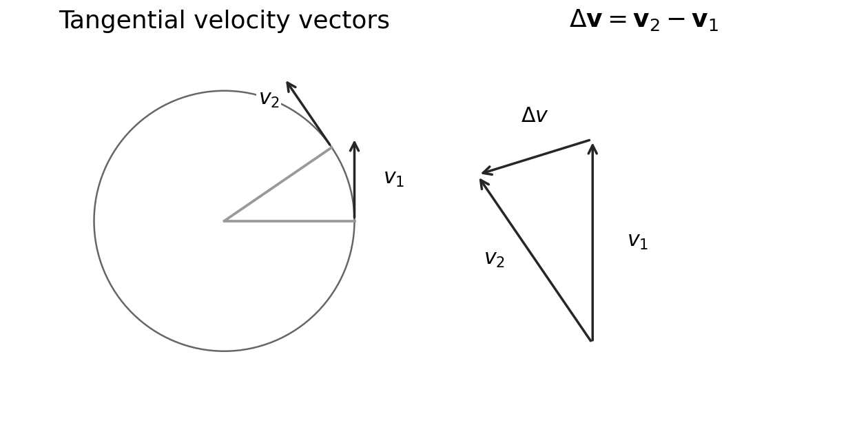
มวลจะตัดกันเพราะทั้งแรงที่ต้องการและแรงที่มีอยู่สเกลตามมวล หากแรงที่ชี้เข้าภายในหายไป การเคลื่อนที่จะเริ่มตามเส้นสัมผัสทันที之后 gravity could curve the later path; “tangent” describes the release direction.
One electronvolt is $e$ joules: $1\ \text{eV}=1.60\times10^{-19}\ \text{J}$ MeV means $10^6$ eV และ GeV means $10^9$ eV มวลที่ถูกquotedใน $\text{MeV}/c^2$ เป็นหน่วยมวล, ไม่ใช่หน่วยพลังงาน คูณด้วย $c^2$ เพื่อรับ rest energy ที่สอดคล้อง与之
หลักฐานความต้องการย้อนกลับ: plans/2026-10-09-edexcel-ial-physics-u5-demand-map.md. การประเมินผล Unit 5 เป็นแบบบูรณาการร่วมกับ Units 1, 2 และ 4
แหล่งที่มา: หลักสูตร Cambridge International
เอกสารประกอบการเรียน
English
From an ice pack to a star
An ice pack, a swinging bridge and a distant star all involve energy. This unit links molecular motion, nuclear changes, oscillations and astronomical observations. The task is often to test a claim, not just calculate a number: state the model, carry units through the calculation, then compare your result with the claim.
WPH15 covers statements 125–171 of Pearson Issue 3. It also uses Units 1, 2 and 4. Work through sheets 5.1–5.9 before their matching authentic sets. Use the supplied constants consistently: $g=9.81\ \mathrm{m\,s^{-2}}$, $k_B=1.38\times10^{-23}\ \mathrm{J\,K^{-1}}$ and $G=6.67\times10^{-11}\ \mathrm{N\,m^2\,kg^{-2}}$ unless the question gives a different local value. Here $k_B$ is the Boltzmann constant; $k_s$ denotes a spring constant.
Heating, phase change and thermistor calibration
Follow the energy, not only the temperature
Internal energy 内能 is the total energy in the random motion and interactions of molecules: random kinetic energy plus intermolecular potential energy. It excludes the kinetic energy of the whole object moving together. Temperature relates to average random molecular kinetic energy, not total internal energy. Two samples at the same temperature can have different internal energies because their amounts and states differ.
Specific heat capacity 比热容$c$ is the energy needed per kilogram for a one-kelvin temperature rise without a change of state. Specific latent heat 比潜热$L$ is the energy transferred per kilogram during a particular change of state at constant temperature.
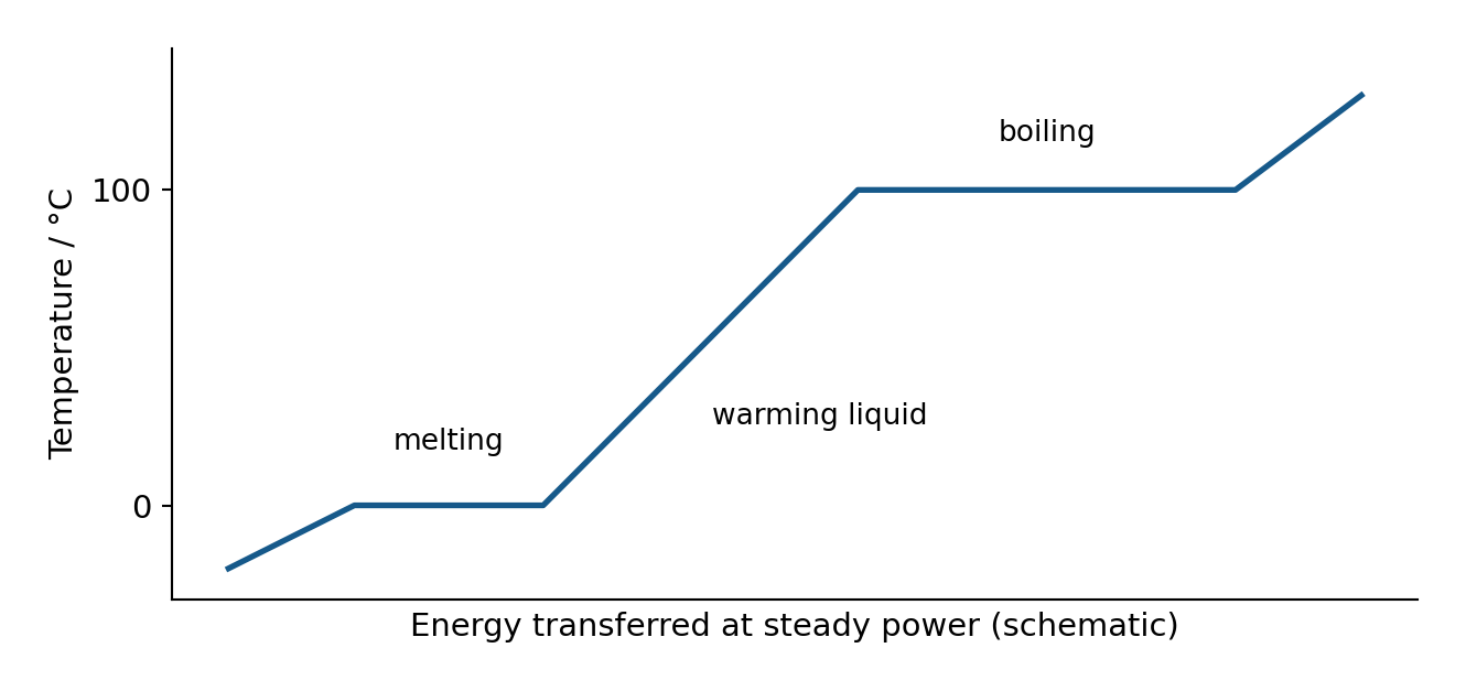
A temperature difference of $1\ ^\circ\mathrm C$ equals a difference of $1\ \mathrm K$. Absolute temperatures in gas and radiation laws must be kelvin. During melting or boiling, energy changes molecular arrangements and potential energy while temperature remains constant in the ideal constant-pressure phase change. An ice pack absorbs energy from the food/surroundings as it melts. It does not send “cold energy” into the food.
At constant heating power, steeper temperature–time gradients mean smaller $mc$, provided heat loss is negligible. A flat section does not mean that energy transfer has stopped. For a heater, input energy is $E_{\rm in}=Pt=VIt$; useful thermal energy can be smaller because energy escapes to surroundings.
Worked example. A $0.40\ \mathrm{kg}$ block of ice at $-10\ ^\circ\mathrm C$ melts to water at $0\ ^\circ\mathrm C$. Use $c_{\rm ice}=2100\ \mathrm{J\,kg^{-1}\,K^{-1}}$ and $L_f=3.4\times10^5\ \mathrm{J\,kg^{-1}}$.
Known: mass, initial/final temperatures and material constants. Why: warming the solid and melting it are separate energy transfers.
Worked example. A $1000\ \mathrm W$ heater boils away $0.20\ \mathrm{kg}$ of water in $600\ \mathrm s$. Find efficiency, using $L_v=2.26\times10^6\ \mathrm{J\,kg^{-1}}$.
For repeated kettle loads, calculate total water volume, number of loads and total operating time. Compare energies over the same stated interval. Standby loss over a day and input needed to boil water are different quantities; state what a particular comparison actually establishes.
CP12: calibrate a thermostat
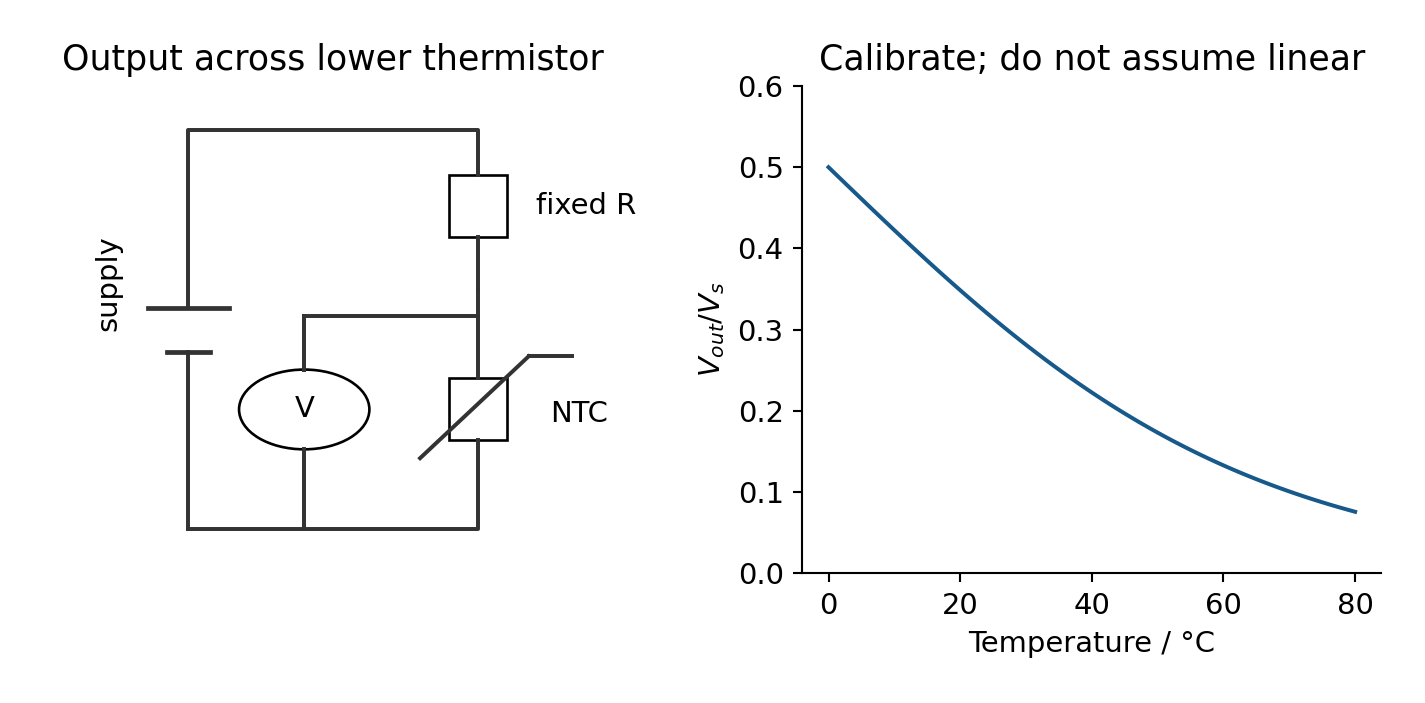
A thermistor 热敏电阻 has resistance that changes with temperature. The usual negative-temperature-coefficient (NTC) thermistor decreases in resistance when heated. In a potential divider 分压器:
With the thermistor as the lower resistor and output measured across it, warming reduces output voltage. Swapping resistor positions reverses that trend. A thermostat switches at a chosen output threshold; the divider alone is not a complete switching device.
For core practical 12, place the thermistor and a reference thermometer close together in a stirred water bath. Keep electrical contacts dry and insulated. At several temperatures across the intended range, wait for thermal equilibrium and record temperature and divider voltage. Keep supply voltage and fixed resistance unchanged. Use a high-input-resistance voltmeter to reduce loading. Plot output against temperature and interpolate the voltage for the chosen switching temperature. Repeat readings or compare warming/cooling to reveal lag. Do not assume a linear calibration without evidence. Use low-voltage electricity and take care with hot water.
CP13: measure latent heat
Supply measured electrical power to a material during its phase change. Measure mass melted or evaporated over a timed interval after conditions stabilise. A balance measures mass change; do not confuse collected liquid volume with mass. Without loss correction, $L=VIt/\Delta m$ assumes all supplied energy causes the phase change.
A useful correction is to compare two powers at the same steady phase-change temperature. If heat-loss power is approximately unchanged, subtracting the two measurements removes it:
$$L=\frac{P_2-P_1}{\dot m_2-\dot m_1}$$
State that constant-loss assumption. A control measurement of melting without the heater is another possible correction in a suitable ice experiment. Reduce heat loss with insulation where safe; avoid splashing, hot surfaces and unsafe mains connections.
Ideal gases and molecular kinetic energy
Kelvin and the ideal-gas model
Absolute zero 绝对零度 is $0\ \mathrm K$, about $-273\ ^\circ\mathrm C$. It is the lower limit of thermodynamic temperature. In the classical ideal-gas model, average translational kinetic energy tends to zero as temperature tends to zero. Real gases condense before that extrapolation is reached; do not claim molecules in every real material lose all possible energy.
Absolute temperature 绝对温度 is measured in kelvin: $T=\theta_{^\circ\mathrm C}+273$ to the precision normally used here. An ideal gas 理想气体 consists of particles with negligible volume, no intermolecular forces except during elastic collisions, and random motion. Pressure comes from momentum changes at walls.
$$pV=Nk_BT$$
Here $N$ is the number of molecules, not the number of moles. Use pressure in pascals, volume in cubic metres and temperature in kelvin. For a fixed number of molecules:
$$\frac{p_1V_1}{T_1}=\frac{p_2V_2}{T_2}$$
At fixed volume, pressure is proportional to kelvin temperature. At fixed temperature, $pV$ is constant. Include external pressure if a gauge reports pressure relative to the atmosphere.
Worked example. A rigid $2.0\times10^{-3}\ \mathrm{m^3}$ vessel contains gas at $1.0\times10^5\ \mathrm{Pa}$ and $300\ \mathrm K$. Find $N$ and pressure after warming to $360\ \mathrm K$.
If one molecule has mass $m_0$, total gas mass is $Nm_0$. For a sphere, first find $V=4\pi r^3/3$; radius is half the diameter.
Derive the molecular energy relation
The kinetic-theory pressure relation is $pV=\tfrac13Nm_0\langle c^2\rangle$, where $\langle c^2\rangle$ is mean square speed 速率平方的平均值. It follows from elastic momentum changes at a wall and equal mean squared motion in the three perpendicular directions. The root mean square speed 方均根速率 is $c_{\rm rms}=\sqrt{\langle c^2\rangle}$; it is not the square of mean speed.
For a cube of side $l$, one molecule with velocity component $c_x$ changes wall momentum by $2m_0c_x$ at each elastic collision. Its return time to that same wall is $2l/c_x$. Hence its average force is $m_0c_x^2/l$. Sum over molecules and divide by wall area $l^2$:
Random motion is equally distributed among perpendicular directions, so $\langle c^2\rangle=3\langle c_x^2\rangle$. This gives the pressure relation above. Equate the two expressions for $pV$, cancel $N$, then rearrange:
At one temperature, different gas species have equal mean translational kinetic energies, but lighter molecules have greater RMS speeds. If speed doubles at the same temperature, molecular mass is one quarter. Heating increases average molecular kinetic energy; it does not give every molecule the same speed.
CP14: pressure and volume at fixed temperature
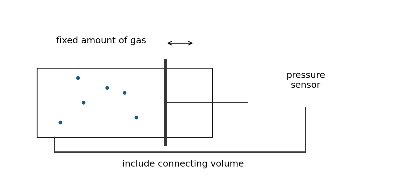
Trap a fixed amount of gas in a syringe or calibrated cylinder connected to a pressure sensor. Check calibration and use absolute pressure. Include connecting-tube dead volume where significant. Change volume gradually, wait after each change for temperature to return to the surroundings, then record several pressure–volume pairs. Do not let gas escape. A plot of $p$ against $1/V$ should be straight through the origin within uncertainty. A $p$–$V$ curve is not straight. Avoid excessive pressure and secure connections. Rapid compression heats the gas and breaks the intended constant-temperature condition.
Binding energy, fission and fusion
Mass deficit is an energy difference
A nucleus contains $Z$ protons and $A-Z$ neutrons. Its mass is smaller than the total mass of these free nucleons. This mass deficit 质量亏损 corresponds to the binding energy 结合能 needed to separate the nucleus completely into free nucleons:
$$\Delta m=Zm_p+(A-Z)m_n-m_{\rm nucleus}\qquad E_b=\Delta m c_0^2$$
Here $c_0$ is the speed of light, distinguished from specific heat capacity. The unified atomic mass unit 统一原子质量单位 is $1\ \mathrm u=1.66\times10^{-27}\ \mathrm{kg}$. Convert all masses to the same unit before subtracting. Nuclear masses and neutral-atom masses are not interchangeable without accounting consistently for electrons. Use the masses the question actually supplies.
$$1\ \mathrm{MeV}=1.60\times10^{-13}\ \mathrm J\qquad \text{binding energy per nucleon}=E_b/A$$
Worked example. A nucleus has mass deficit $0.030\ \mathrm u$ and $A=4$. Find binding energy per nucleon.
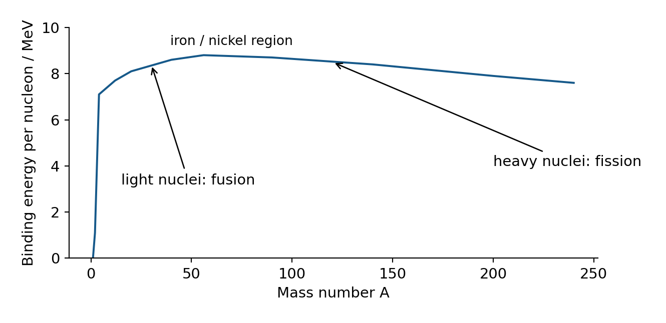
The binding-energy-per-nucleon curve rises steeply for light nuclei, peaks near iron/nickel, then decreases gradually for heavy nuclei. Greater binding energy per nucleon generally means nucleons are more tightly bound. It is the vertical value, not just mass number, that matters when comparing points.
Nuclear fusion 核聚变 combines light nuclei. Nuclear fission 核裂变 splits a heavy nucleus into smaller products, often with neutrons. Energy is released when the products have greater total binding energy and smaller total rest mass than the reactants. For a reaction, calculate the total mass difference, not merely a difference of two per-nucleon values. Total energy is conserved.
Fusion needs very high temperature to give nuclei enough kinetic energy to approach despite electrostatic repulsion, and high density/confinement to make enough close encounters and sustain energy release. Temperature and density have different roles. Merely naming “high pressure” does not explain overcoming repulsion.
Radiation, background and decay
Choose radiation by its interaction
Alpha radiation 阿尔法辐射 consists of helium nuclei: strongly ionising, short range and stopped by paper or a few centimetres of air. Beta radiation 贝塔辐射 consists of electrons or positrons: less ionising, more penetrating, typically stopped by a few millimetres of aluminium. Gamma radiation 伽马辐射 is electromagnetic radiation: weakly ionising and highly penetrating; lead or concrete reduces its intensity but does not provide a sharp stopping thickness.
In a cloud chamber, alpha tracks are thick mainly because of strong ionisation, and relatively straight because the particles have large mass compared with beta particles. Beta tracks are thinner and more easily deflected. Do not swap these explanations. Beta radiation can monitor paper thickness because some passes through and some is absorbed; a change in thickness changes the transmitted count rate.
In nuclear equations 核反应方程, conserve nucleon number and charge number. Beta-minus decay converts a neutron to a proton; the mass number stays the same and atomic number increases by one. Include the antineutrino where required, as in Unit 4:
Alpha decay reduces $A$ by four and $Z$ by two. Gamma emission changes neither $A$ nor $Z$. Nuclear equations conserve more than these two numbers: energy and momentum still matter.
Correct background before applying a model
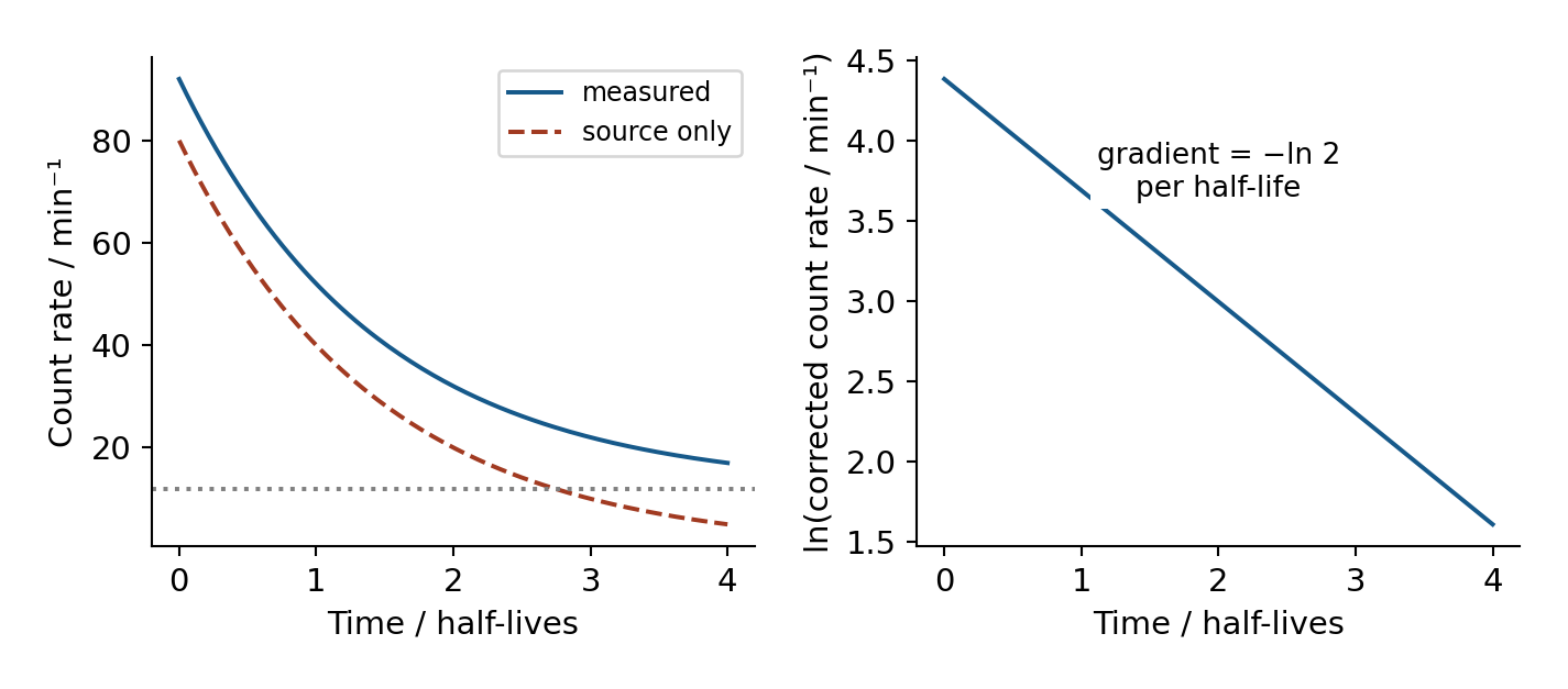
Background radiation 本底辐射 comes from sources such as rocks, cosmic rays and the environment. Measure it for a sufficiently long time with the test source absent. Subtract its count rate from every source-plus-background reading. Keep counting-time units consistent. Corrected detector count rate is proportional to source activity only when geometry and detection efficiency remain unchanged; it is not automatically the activity in becquerels.
Worked example. A detector reads $62\ \mathrm{min^{-1}}$ at distance $r$, including background $14\ \mathrm{min^{-1}}$. Predict total rate at $2r$ for a small isotropic gamma source with negligible absorption.
Do not divide the background by four: it is not all coming from the test source.
Random events, predictable populations
Radioactive decay 放射性衰变 is spontaneous: an unstable nucleus decays without an external trigger. It is random: the exact time for an individual nucleus cannot be predicted. A large population has a predictable statistical decay pattern. Activity 放射性活度$A$ is the number of decays per second, measured in becquerels 贝可勒尔, $1\ \mathrm{Bq}=1\ \mathrm{s^{-1}}$.
The decay constant 衰变常数$\lambda$ is the probability per unit time of decay for a nucleus. The half-life 半衰期$t_{1/2}$ is the time for the undecayed population, or activity, to halve on average.
At one half-life, $N/N_0=1/2=e^{-\lambda t_{1/2}}$. Taking logs gives:
A log-activity–time line has gradient $-\lambda$. Take logarithms of corrected rates, not source-plus-background readings. Read several half-life intervals from a graph and average; measure from the corrected activity level, not from zero total counts.
Worked example. A source has half-life $3.0\ \mathrm{years}$. When will activity fall to $2.0\%$ of its initial value?
Use a fraction, not $2.0$ inside the logarithm. If calculating power from a radioactive source, $P=A E_{\rm decay}$, with energy per decay in joules. This is released nuclear power; useful electrical output may be smaller. Convert the half-life to seconds when activity must be in becquerels.
CP15: absorption of gamma radiation by lead
Keep source, absorber and detector in fixed positions. Measure background, then counts over equal known intervals for several total lead thicknesses. Repeat or extend the counting time because counts fluctuate. Subtract background rate before comparing transmission. If each equal thickness gives the same fractional reduction, the attenuation is exponential; a graph of log corrected rate against thickness is approximately straight. Three half-value thicknesses transmit $1/8$, not $1/3$.
The material-absorption constant is not the time-decay constant of the source. Avoid readings too close to background, where subtraction gives large relative uncertainty. Handle sources with the specified tools under supervision, keep distance, minimise exposure time and return them to shielding. Never touch a source or direct it at people. Keep lead handling clean and wash hands.
Simple harmonic motion, graphs and energy
The restoring condition
Simple harmonic motion 简谐运动 (SHM) occurs when resultant acceleration is proportional to displacement from a fixed equilibrium position and directed towards it:
The negative sign is the restoring direction. Constant speed, repetition alone or a force merely pointing towards a centre does not establish SHM. For a vertically hanging spring, measure $x$ from the loaded equilibrium position. Weight is already balanced there; the resultant for displacement is $-k_sx$.
For release from positive maximum displacement at $t=0$:
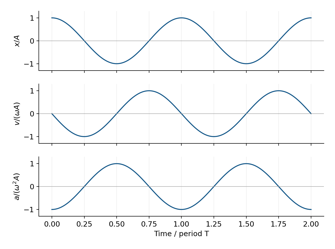
Here $A_0$ is amplitude, not radioactive activity. The phase depends on the chosen starting time; a sine displacement can describe the same motion with another origin. Differentiate graphically: the displacement–time gradient is velocity, and velocity–time gradient is acceleration. At maximum displacement, speed is zero and acceleration points back towards equilibrium. At equilibrium, speed is greatest and acceleration is zero.
Worked example. A graph gives amplitude $0.030\ \mathrm m$ and period $0.50\ \mathrm s$. Find maximum speed and acceleration.
Alternatively find maximum speed from a tangent to the displacement graph at equilibrium. Convert centimetres to metres. A negative straight $a$–$x$ gradient is $-\omega^2$, so take its negative before the square root.
Periods and energy
For a mass on an ideal spring and for a simple pendulum at small angles:
Pendulum length is pivot to bob centre. The small-angle period does not depend on bob mass. A period ratio for one unchanged spring gives $T_2/T_1=\sqrt{m_2/m_1}$. Use total new mass before finding added mass.
Worked example. A $0.50\ \mathrm{kg}$ mass has period $0.80\ \mathrm s$. An extra mass increases the period to $1.00\ \mathrm s$ on the same spring.
Thus the $E_k$–$x$ graph is an inverted parabola: zero at $\pm A_0$, positive maximum at $x=0$. The $E_p$–$x$ graph opens upwards. Their sum is constant in the undamped model. In a damped system energy is transferred out, so amplitude decreases. Total energy including surroundings remains conserved.
CP16: infer an unknown mass from resonance
Keep the same spring/support system. Attach several known masses, drive with small oscillations and vary frequency to find the largest steady amplitude for each mass. Record the resonant frequency, repeating slowly around each peak. With light damping it approximates natural frequency. Plot $1/f^2$ against total known mass; the spring model gives gradient $4\pi^2/k_s$. Use the calibration to infer an unknown mass from its resonant frequency.
Account for a hanger and, where significant, the effective moving mass of the spring. A nonzero intercept may represent this contribution; do not force the line through the origin without justification. Keep amplitudes small and below the elastic limit. Secure masses and stand, and keep feet clear. Measuring free periods can provide a useful independent comparison, but the specified practical uses resonant frequencies.
Forced oscillations, resonance and damping
A free oscillation 自由振动 follows an initial disturbance without continued periodic driving. A forced oscillation 受迫振动 is maintained by a periodic driving force; its steady frequency is the driving frequency. Natural frequency 固有频率 is the frequency of free oscillation for the system under the stated conditions.
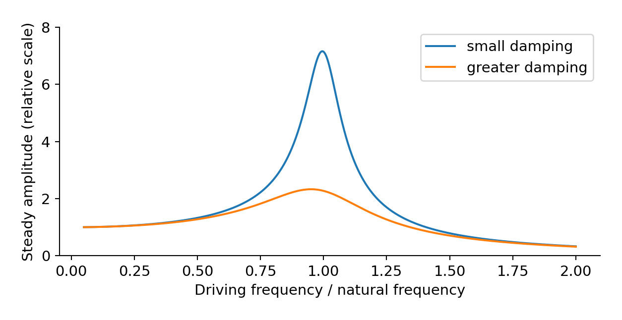
Resonance 共振 occurs when driving frequency is at or near natural frequency, giving efficient energy transfer and a large steady amplitude. It does not mean “maximum frequency”. For a lightly damped system, the amplitude peak is near the undamped natural frequency. Greater damping lowers and broadens the peak; do not present every damped peak as exactly at the undamped natural frequency.
Damping 阻尼 transfers energy away from oscillation, for example through resistive work that increases the thermal energy of dampers and surroundings. Stronger damping can reduce dangerous bridge/building motion. Plastic deformation 塑性形变 of a ductile material also absorbs mechanical energy irreversibly; purely elastic deformation returns stored energy and is not the same mechanism.
Worked explanation. People walking supply a periodic driving force to a bridge. If its frequency is near a natural frequency, energy transfers efficiently into the bridge and amplitude increases. Dampers do work against motion, transferring oscillation energy to thermal stores, so the steady amplitude is limited. Link cause and effect in this order rather than listing “resonance, energy, damping”.
For the same shape and amplitude, adding mass to a light pendulum increases its stored mechanical energy while the small-angle ideal period remains unchanged. Under comparable resistive losses it can lose a smaller fraction of energy per cycle. That contextual damping comparison does not prove that every heavier oscillator always damps more slowly.
Gravitational fields and orbits
Field and potential have different meanings
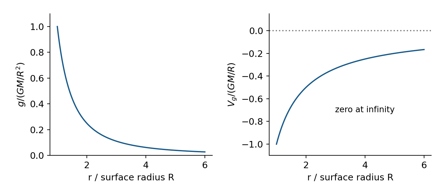
A gravitational field 引力场 is a region where a mass experiences a force. Gravitational field strength 重力场强度$g=F/m$ is force per unit test mass. It is a vector pointing towards an isolated source mass. Newton's law for point masses, or outside a spherical symmetric source, is:
$r$ is centre-to-centre distance, not height above the surface. For near-Earth local motion, constant $g$ can be suitable. Over large radial distances it is not constant.
Gravitational potential 引力势 is potential energy per unit mass, with zero at infinity:
Potential is a scalar and negative at finite distance. Moving outward makes it less negative, so potential energy increases while attractive force weakens. A potential graph value and its corresponding radius give $M=-Vr/G$.
Gravity and electric fields are both radial for isolated point sources and their force magnitudes obey inverse-square laws. Gravity acts on mass and is attractive in this model. Electric force acts on charge and can attract or repel. Electric field direction follows the force on positive test charge; a negative charge is forced oppositely.
Worked example. A $1000\ \mathrm{kg}$ satellite moves from radius $r_1=6.4\times10^6\ \mathrm m$ to $r_2=1.28\times10^7\ \mathrm m$ around Earth, $M=6.0\times10^{24}\ \mathrm{kg}$. Find its potential-energy change.
The positive sign is final minus initial. This is not the total launch energy, since kinetic energy may also change. $mg\Delta h$ with constant surface $g$ is unsuitable over this distance.
Derive a circular orbit
The gravitational force supplies the inward resultant:
Orbiting mass cancels. The period grows with radius. To appear stationary above one point on a rotating planet, a satellite needs a circular equatorial orbit, the same rotational direction and matching angular velocity/period. Matching period alone is insufficient.
Worked example. For $GM=4.00\times10^{14}\ \mathrm{m^3\,s^{-2}}$ and period $T=8.64\times10^4\ \mathrm s$, find stationary-orbit radius.
Subtract planet radius only if asked for height above the surface. For a star's surface field, use its radius, not its listed diameter; test a multiple-of-Earth-field claim by calculating the ratio.
Stellar radiation, distances and evolution
Temperature, luminosity and received intensity
A black body 黑体 absorbs all incident electromagnetic radiation and is an ideal thermal emitter. Its continuous spectrum has a characteristic shape. Increasing temperature increases total emitted power per unit area and moves the wavelength peak to shorter wavelength. The area under a spectral-intensity curve represents total intensity only with the appropriate spectral-axis definition.
Luminosity 光度$L_\star$ is total power emitted. Intensity 强度$I$ received at distance $d$ is power per unit receiving area. For a spherical black-body star of radius $R$ radiating equally in all directions:
The first area is the emitting surface; the second is the expanding receiving sphere. Do not substitute observer distance into the star's surface area. Real emitters may not be perfect black bodies, and intervening material can absorb radiation.
Wien's stated constant describes a spectrum per unit wavelength. A maximum of a spectrum plotted per unit frequency does not transform into that wavelength maximum simply by replacing $\lambda$ with $c_0/f$. If an exam gives the frequency corresponding to its specified wavelength peak, convert that given wavelength using $c_0=f\lambda$. Do not turn that particular task convention into a general rule for every spectral plot.
Worked example. A star's wavelength spectrum peaks at $580\ \mathrm{nm}$ and its radius is $7.0\times10^8\ \mathrm m$. Find temperature, luminosity and intensity at $1.5\times10^{11}\ \mathrm m$.
Keep unrounded temperature because it is raised to the fourth power. Compare the received intensity with the stated reference before accepting a planetary-temperature or power claim.
Two distance methods
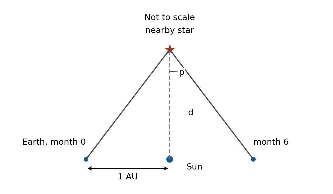
Trigonometric parallax 三角视差 measures a nearby star's apparent angular shift against distant background stars as Earth moves around the Sun. Observations six months apart use a baseline of two Earth-orbit radii. The parallax angle $p$ is half the total shift. For small $p$ in radians, distance is $d\approx r_{\rm orbit}/p$. A parsec 秒差距 is the distance giving parallax $1$ arcsecond; $d_{\rm pc}=1/p_{\rm arcsec}$. Do not use the diameter of Earth or Sun as the orbital baseline.
At large distance, $p$ becomes too small for the instrument to measure accurately. The limitation is angular resolution/relative uncertainty, not necessarily that the star is invisible.
A standard candle 标准烛光 is an object of known luminosity. Identify one in a cluster, measure received intensity and use $d=\sqrt{L_\star/(4\pi I)}$. Its apparent brightness is not assumed known beforehand. Cepheid variable stars have a calibrated relationship between period and luminosity. Measure several complete light-curve periods, divide by their number, read the calibration carefully and convert any solar-luminosity units. A straight line on log axes is not automatically a linear relationship between the raw quantities.
Worked example. A standard candle has $L_\star=4.0\times10^{28}\ \mathrm W$ and received intensity $2.0\times10^{-10}\ \mathrm{W\,m^{-2}}$.
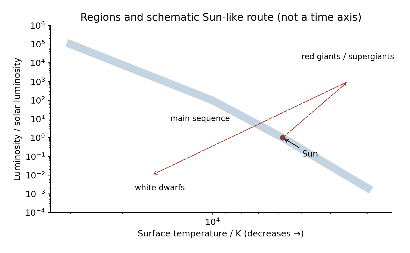
A Hertzsprung–Russell diagram 赫罗图 plots luminosity vertically against surface temperature horizontally, usually with temperature decreasing to the right and logarithmic scales. The main sequence 主序星带 runs from hot, bright stars at upper left to cool, faint stars at lower right. Red giants 红巨星 are cool but luminous because of their large surface areas. White dwarfs 白矮星 are hot but faint because of their small surface areas. Mark the Sun near one solar luminosity and about $5800\ \mathrm K$ on the main sequence.
Stars form when gravity contracts a cloud of gas and dust. The core heats until hydrogen fusion can sustain a main-sequence star; outward pressure balances gravity. In a Sun-like star, core hydrogen eventually runs low, fusion there decreases and gravity contracts the core. Core temperature rises; shell hydrogen burning and later helium fusion are associated with expansion to a red giant. Outer layers are lost, leaving a white-dwarf core with no sustained fusion. It cools over a very long time. The Sun does not become a supernova or a neutron star.
A much more massive star can fuse heavier elements through later stages. When its core can no longer gain energy from fusion, collapse and a supernova can leave a neutron star or black hole, depending on the remnant. A massive main-sequence star has more fuel but consumes it much faster because of its hotter core. Its main-sequence lifetime can therefore be shorter. Explain fusion rate, not just fuel amount. An HR track shows changing temperature/luminosity, not a star travelling across space.
Doppler shifts and cosmology
Compare the same spectral line
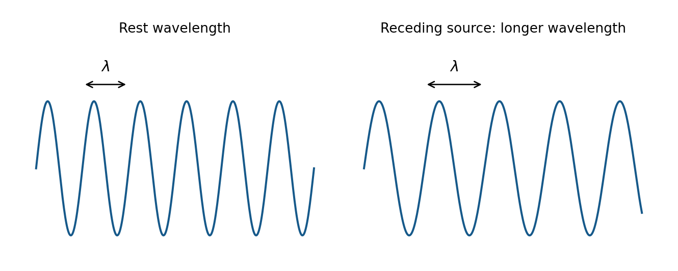
The Doppler effect 多普勒效应 is a change in observed frequency/wavelength caused by relative motion along the line of sight. Successive wavefronts arrive farther apart from a receding source and closer together from an approaching source. Recession gives longer wavelengths and lower frequencies; approach gives shorter wavelengths and higher frequencies. Motion purely perpendicular to the line of sight is not the recession speed in the simple model.
For electromagnetic radiation at low recession speeds:
Redshift 红移$z$ is positive for recession. For small shifts, its magnitude also approximately equals the fractional decrease of observed frequency relative to emitted frequency. State the sign convention: $(f_{\rm observed}-f_{\rm rest})/f_{\rm rest}$ is negative for recession. Do not equate a positive redshift to a signed frequency increase. The approximation $v/c_0$ is not a general high-speed relativistic formula.
Worked example. A line emitted at $500\ \mathrm{nm}$ is observed at $505\ \mathrm{nm}$.
To use a star's absorption lines, recall Unit 2: photons are absorbed only when their energies match allowed atomic-level differences. Compare the same identified spectral line, not two different elements.
For opposite limbs of a rotating star, one approaches while the other recedes. If their shifts are equal and opposite, the separation of the two observed wavelengths is twice the shift of either limb. Halve that separation before finding the equatorial speed. Then use $T=2\pi R/v$. This assumes the observed line-of-sight limb speed represents the equatorial rotation speed under the stated viewing geometry.
Hubble law and its limits
On large cosmological scales, recession speed approximately follows Hubble's law 哈勃定律:
$$v=H_0d$$
The Hubble constant 哈勃常数$H_0$ has units of inverse time. In $\mathrm{km\,s^{-1}\,Mpc^{-1}}$, convert kilometres to metres and megaparsecs to metres before taking its reciprocal in seconds. Nearby objects may have local motions that do not follow the large-scale relationship.
Worked example. Use $H_0=70\ \mathrm{km\,s^{-1}\,Mpc^{-1}}$ and $1\ \mathrm{Mpc}=3.1\times10^{22}\ \mathrm m$ to estimate an expansion timescale.
The reciprocal is the Hubble time 哈勃时间. Interpreting it as an age assumes a model for the past expansion rate; it is not an exact model-independent age. A larger $H_0$ gives a smaller reciprocal timescale. Evidence for expansion supports an earlier denser, hotter universe; it does not describe an explosion into an already empty centre-surrounding space.
Dark matter 暗物质 is inferred from gravitational effects that visible matter alone does not explain, such as galaxy rotation and motion. It need not emit detectable light. The amount of gravitating matter affects how expansion changes, so uncertainty in matter content and the expansion model affects predictions of the universe's fate. Do not infer that one measurement of $H_0$ alone proves perpetual expansion or future collapse. Modern models also consider dark energy; outcome 171 specifically requires understanding the controversy concerning $H_0$, dark matter, age and fate, rather than memorising one unqualified prediction.
Check yourself
Why can internal energy increase without temperature increasing during a phase change?
A fixed amount of gas warms in a rigid vessel. Which temperature scale must be used to compare pressures?
Does greater binding energy per nucleon mean that less or more energy is needed to separate each nucleon on average?
Why must background be subtracted before using a count-rate ratio or logarithm?
An $a$–$x$ line has gradient $-25\ \mathrm{s^{-2}}$. Find angular frequency.
Why is maximum SHM speed at equilibrium although acceleration is zero there?
Why can a damped bridge be driven at the same frequency but oscillate with a smaller amplitude?
Does lifting a satellite to a larger radius increase or decrease its signed gravitational potential energy?
A star is hot but faint. Which HR region is plausible, and what can explain its low luminosity?
When using the wavelength separation of opposite rotating limbs, why is a factor of two needed?
Answers: (1) molecular potential energy changes; (2) kelvin; (3) more; (4) background does not follow the source's decay/distance law; (5) $\omega=\sqrt{25\ \mathrm{s^{-2}}}=5.0\ \mathrm{rad\,s^{-1}}$; (6) restoring resultant is zero there but energy is mostly kinetic; (7) greater energy loss limits steady amplitude; (8) increases towards zero; (9) white dwarf, small emitting surface; (10) one limb is blueshifted while the other is redshifted.
Two students measure the same damped pendulum. One records amplitudes; the other records amplitudes, processes them with logarithms, draws one straight line and reads off a decay constant and an initial amplitude. The second student has turned raw readings into a result. Unit 6 tests exactly that step.
WPH16 Practical Skills in Physics II is a written paper about the experiments you met while studying Units 4 and 5: gas laws, capacitors, damped oscillations, radioactive decay, light intensity. It lasts 80 minutes and has 50 marks. All questions are compulsory, and at least 20 marks use Level-2 mathematics. A written guide supports real laboratory work; it does not replace carrying out experiments yourself.
The four skill sheets follow the paper's own flow: plan the investigation, carry it out and judge the measurements, then process the data with uncertainties and graphs.
A valid measurement 有效测量 still means measuring what you intend to measure. At A2 the plan has one extra demand: decide how the data will be processed before writing the method. The graph you intend to draw decides how many readings you need and where you take them.
Choose the graph before the method
Suppose you must test a predicted relationship. Work backwards:
Write the model, for example $P = kX^4$ or $A = A_0\mathrm{e}^{-\lambda n}$.
Rearrange it into the straight-line form $y = mx + c$. This step is linearisation 线性化: choose a plot such as $P$ against $X^4$, $\ln A$ against $n$, or $\lg P$ against $\lg X$.
State what the graph proves: a straight line through the origin for $P$ against $X^4$, or gradient 斜率$4$ on the log graph 对数图像 of $\lg P$ against $\lg X$.
Then choose the readings: at least five well-spread settings of the quantity you change.
A plan without its graph is an unfinished plan. The paper's six-mark "devise a method" questions expect the graph to appear in the answer.
Worked planning example: absolute zero from a gas flask
A flask of fixed air volume carries a pressure gauge and a thermometer. Predict how to estimate absolute zero.
Known aim: the pressure of a fixed mass of gas falls linearly with temperature and reaches zero at absolute zero. Why this route: the zero-pressure point cannot be reached in water baths, but a straight line can be extended to it.
Use a beaker of water with ice for $0\ ^\circ\mathrm{C}$ and a hot plate (or Bunsen burner) to raise the temperature to boiling. Stir so the water shares one temperature.
Place the thermometer close to the flask, on the side away from the heater, and read the scale perpendicular to it.
Record paired pressure and temperature readings at a minimum of five temperatures, spaced no more than about $20\ ^\circ\mathrm{C}$ apart. These are new settings, not repeats of one setting.
Plot pressure against temperature in $^\circ$C, draw the best-fit line 最佳拟合线 and extrapolate 外推 it to $p = 0$. The intercept 截距 on the temperature axis estimates $-273\ ^\circ$C.
Extrapolation extends a straight line beyond the measured range; the measured points themselves stay between ice and boiling water.
The extrapolated answer depends on the fitted line, so scatter matters more here than in a single reading. That is the price of a point you cannot measure directly.
Worked planning example: testing a power law
A light sensor a fixed distance from a filament bulb reads $X$; the electrical power is predicted to follow $P = kX^4$.
Control what else changes $X$: keep the bulb-sensor distance and alignment fixed, and work in a darkened space so background light does not add to the reading.
Measure the current $I$ and potential difference $V$ at each setting, and calculate $P = IV$.
Take at least five settings by changing the current, then choose one of two graphs:
$$\lg P = \lg k + 4\lg X \qquad \text{or} \qquad P = k\,(X^4)$$
A graph of $\lg P$ against $\lg X$ should be straight with gradient $4$. A graph of $P$ against $X^4$ should be straight through the origin. Either answers the question; name the expected gradient or origin when you claim the test.
A power law becomes a straight line on log/log axes; the gradient is the power.
The specification's own example is a gas: plot an appropriate log/log graph of pressure against volume for a fixed mass at constant temperature. Log graphs are not only for exponential decay.
Circuits that measure what the investigation needs
An investigation of a component needs both meters in the right places:
an ammeter 电流表 in series with the component, so the same current flows through it;
a voltmeter 电压表 in parallel with the component under test only, so it reads that component's potential difference;
a way of changing the current: a variable resistor or potentiometer, in series with a fixed supply.
If the voltmeter straddles two components, the reading no longer belongs to the thing you are investigating. When a two-position switch moves a charged capacitor to a new circuit, draw the voltmeter across the one capacitor the question names, and connect the second capacitor in parallel with it.
Electrolytic capacitors add their own safety rules: connect with the correct polarity, keep the supply below the working voltage, and discharge the capacitor before handling it.
Data loggers and safety, with reasons
A data logger 数据采集器 with probes records pairs of readings at the same moment, removes parallax 视差 from scale reading, and its probes usually have a better resolution 分辨率 than a liquid-in-glass thermometer. Say which of these changes improves the measurement; "more accurate" alone names no mechanism.
Safety answers follow the same rule: name the hazard and the action. Hot water and immersion heaters burn — move glass with tongs or heat-proof gloves, and clamp the heater so its leads cannot topple the beaker. Switch off before removing anything electrical.
A damped pendulum swings past a rule, and its turning points move quickly. Judging the amplitude to the nearest $1\ \text{mm}$ claims a precision the eye cannot deliver, especially viewing the scale at an angle or with the bob far from the rule. Recording to the nearest $5\ \text{mm}$ matches the recording to what can honestly be judged.
This is a two-way skill: criticise a recording resolution that is too fine, and justify a coarse one with the reason it is appropriate.
Timing oscillations
Measure the time for many oscillations, then divide. The reaction-time uncertainty is nearly the same whether you time one swing or ten, so a larger measured time gives a smaller percentage uncertainty in the period.
Two techniques earn marks on their own:
put a timing marker 计时标记 at the centre of the oscillation and time passes through it, because the mass moves fastest there and the moment of passing is clearest;
start the timer only after several oscillations, when the motion has settled, and use a small initial displacement.
For the period itself, record repeats of the total time, take the mean, and only then divide by the number of swings.
Length instruments at A2
The Unit 3 techniques still earn the marks, now with reasons attached:
measure a spring or cylinder diameter with calipers at several orientations 方位 around the coil or cross-section and average, because a real object is not perfectly round (this attacks random variation 随机变化);
check the zero reading with the jaws closed and subtract a zero error, because it shifts every reading the same way (this attacks a systematic error 系统误差);
use the micrometer ratchet so the jaws tighten the same amount each time.
Justifying an instrument is quantitative: a micrometer resolves $0.01\ \text{mm}$, so a single $1.21\ \text{mm}$ slide has an uncertainty of $0.005\ \text{mm}$. Its percentage uncertainty 百分比不确定度 is:
A small percentage uncertainty is the justification; "it is accurate" is not.
Criticising tables and graphs
For a table of results, check:
significant figures 有效数字: raw readings use the same decimal places as the instrument's resolution; processed values for plotting are commonly $3$ significant figures. A column mixing $5.1$ with $5.143$ has a fault to name.
units: every column heading carries its unit, once, in the heading.
values that stand outside the pattern of the others, judged against the graph as well as the table.
For a plotted graph, the examiner's checklist is short:
enough data points, spread over more than half of each axis, on scales that are not awkward (multiples of $3$ or $7$ are hard to read);
points plotted to within $1\ \text{mm}$ (half a small square);
a thin, continuous best-fit line that balances the scatter;
whether the points actually support a straight line at all.
Criticising a graph is not listing everything you know. Point at the actual defect: five points crowded into a quarter of the grid, or a gentle curve drawn as a line.
Unit 6 expects compounded uncertainties 复合不确定度, which Unit 3 did not. The rules come from the specification's Appendix 10.
The building blocks
A single reading has an uncertainty of half the instrument's resolution. Repeated readings have an uncertainty of half the range (the reading furthest from the mean is an accepted alternative). A percentage uncertainty is:
Quote percentage uncertainties to one or two significant figures. Halving or doubling a measured quantity leaves its percentage uncertainty unchanged, which is why percentages, not absolute values, are the working currency.
The three compounding rules
A power multiplies the percentage uncertainty. If $A = \pi r^2$ and $r$ has $0.6\%$ uncertainty, then $A$ has $2\times0.6\% = 1.2\%$. A diameter and its radius share the same percentage uncertainty.
Products and quotients add percentage uncertainties. Density $\rho = m/l^3$ from $m$ with $0.1\%$ and $l$ with $2.1\%$ gives $3\times2.1\%+0.1\% = 6.4\%$.
Sums and differences add absolute uncertainties. Subtracting two heights measured to $\pm0.5\ \text{mm}$ each gives $\Delta h = \pm1\ \text{mm}$, even though the heights themselves are several hundred millimetres.
The third rule is why differences of similar measurements carry large percentage uncertainties, and it combines with the first two: the percentage uncertainty of $D^2/(2d^2)$ is $2\times\%U(D) + 2\times\%U(d)$.
Worked example: the ramp measurement of g
A sphere rolls a distance $s$ down a ramp of height difference $\Delta h$ in time $t$, where:
$$t^2 = \frac{14s^2}{5g\,\Delta h} \qquad\Rightarrow\qquad g = \frac{14s^2}{5t^2\Delta h}$$
Known: $s = 90.0\ \text{cm}\pm0.1\ \text{cm}$, $\Delta h = 21\ \text{mm}\pm1\ \text{mm}$, $t = 3.36\ \text{s}\pm0.03\ \text{s}$. Why these rules: $s$ and $t$ are squared (powers), and the quantities are multiplied and divided.
Both routes end in a sentence that states what the evidence supports. A value of $\nu = 0.276\pm6\%$ spans $0.259$ to $0.293$; a data-book $0.265$ for steel falls inside, so the spring could be steel. That is the honest strength of the claim — the interval does not prove it is steel, only that steel is not excluded.
กราฟ log และการทำให้เป็นเชิงเส้น (ส่วนสเปกซิฟิเคชัน 6.5 หัวข้อกราฟ พร้อมส่วน 6.1): ทำให้ความสัมพันธ์เอ็กซ์โพเนนเชียลเป็นเชิงเส้นด้วยลอการิทึมธรรมชาติ (ln y = ln y0 − kt form) รวมถึงหน่วยและเครื่องหมาย; ทำให้กฎกำลัง y = kx^n เป็นเชิงเส้นโดยพล็อต lg y เทียบกับ lg x (ความชัน n, จุดตัดแกน lg k) หรือโดยการพล็อตเทียบกับ x^n; ประมวลผลข้อมูลให้เป็นทศนิยมสามตำแหน่งอย่างสม่ำเสมอสำหรับการพล็อต; ป้ายแกน log ด้วยปริมาณที่ถูกล็อกที่แท้จริง; พล็อตด้วยสเกลที่เหมาะสม, วาดเส้น Best-fit และคำนวณความชันจากสามเหลี่ยมขนาดใหญ่; แปลงความชันหรือจุดตัดกลับเป็นปริมาณทางฟิสิกส์ (เช่น e ยกกำลังจุดตัด); ใช้ความสัมพันธ์ที่ fits เพื่อทำนายสภาวะใหม่ (จำนวนสไลด์จำนวนเต็ม, การลดเป็นเปอร์เซ็นต์); ตัดสินความถูกต้องของการ extrapolate จากความกระจัดกระจาย, ข้อผิดพลาดระบบที่อาจเกิดขึ้น หรือขาดแคลนข้อมูลใกล้จุดตัด
แหล่งที่มา: หลักสูตร Cambridge International
English
Straighten an exponential with ln
A damped pendulum's amplitude follows $A = A_0\mathrm{e}^{-\lambda n}$, where $n$ counts oscillations. Take the natural logarithm of both sides:
$$\ln A = \ln A_0 - \lambda n$$
Compare this with $y = c + mx$: a graph of $\ln A$ against $n$ is straight, with gradient $-\lambda$ and intercept $\ln A_0$. The minus sign is part of the physics — amplitude decays, so the line slopes down.
Worked example. The line's intercept is $2.295$ and its gradient is $-0.0355$.
Known: intercept $=\ln A_0$, gradient $=-\lambda$. Why: $A$ was measured in centimetres, so $\ln(A/\text{cm})$ was plotted.
$\lambda$ has no unit because $n$ is a count. Had $n$ been time in seconds, $\lambda$ would carry $\text{s}^{-1}$.
Processing discipline: compute $\ln$ of every value to a consistent $3$ decimal places, label the axis with the exact quantity logged — $\ln(A/\text{cm})$, not "$\ln A$" with a unit bolted on — and take the gradient from a large triangle 大三角形 covering more than half the drawn line, using points on the line rather than data points off it.
When the intercept is an extrapolation
$A_0$ sits at $n = 0$, where there is no data if the first reading was taken at $n = 5$. The intercept is then only as good as the fitted line:
large scatter leaves the best-fit line uncertain, moving the intercept;
a systematic error in amplitude shifts the whole line;
the pendulum's first swings may not follow the model (a large starting angle stretches the period and distorts early amplitudes).
"Extrapolating beyond the data assumes the model still holds" is the sentence that earns the mark. Say which of these applies to the experiment in front of you.
Use the fitted line to predict
A fitted relation answers questions the raw table cannot. If $\ln V = \ln A - Bw$ for light passing through glass, and the line gives $B = 0.0104\ \text{mm}^{-1}$, the thickness $w$ needed to dim a reading to $75\%$ follows without touching the apparatus again:
With slides of $1.22\ \text{mm}$ each, that is $27.7/1.22 = 22.7$, so $23$ slides — round up, because $22$ slides would not reach the required dimming. Prediction questions test the direction of the final rounding as much as the algebra.
Straighten a power law with lg
For $y = kx^n$, taking base-10 logarithms gives:
$$\lg y = \lg k + n\lg x$$
A graph of $\lg y$ against $\lg x$ is straight with gradient $n$ and intercept $\lg k$. Use it when no power of $x$ makes a convenient linear axis, and keep the base consistent: $\lg$ for the power-law plot, $\ln$ for the exponential one. Both operate on the number after the unit is divided out, so the axis label is $\lg(P/\text{W})$, never $\lg P$ with watts attached.