Discrete random variables
Introduced| English | Meaning |
|---|---|
| discrete random variable/dɪˈskriːt ˈrændəm ˈveərɪəbl/ | A numerical outcome of a random experiment with a finite or countably infinite set of possible values. |
| expectation/ekspɪkˈteɪʃn/ | The probability-weighted average value of a random variable. |
| variance/ˈveərɪəns/ | A measure of spread based on the squared deviations of values from their mean. |
| probability distribution/ˌprɒbəˈbɪlɪti ˌdɪstrɪˈbjuːʃn/ | A description assigning probabilities to the possible values or ranges of a random variable. |
| binomial distribution/baɪˈnəʊmɪəl ˌdɪstrɪˈbjuːʃn/ | A probability model for the number of successes in a fixed number of independent trials with the same success probability. |
| trial/ˈtraɪəl/ | trial |
| geometric distribution/ˌdʒiːəʊˈmetrɪk ˌdɪstrɪˈbjuːʃn/ | A probability model for the number of independent trials up to and including the first success, with constant success probability. |
The loaded die
- A fair die gives each face probability $\dfrac{1}{6}$. But what if the die is loaded? Each outcome still has a probability, but they're no longer equal.
- A discrete random variable 离散型随机变量 assigns a probability to each possible outcome — the foundation of statistical modelling.
Discrete random variables
- A discrete random variable $X$ takes separate values, each with a probability (they sum to 1).
- Expectation 期望 (mean): $E(X) = \sum x\,P(X = x)$.
- Variance 方差: $\text{Var}(X) = \sum x^2\,P(X = x) - \big(E(X)\big)^2$.
Worked example. $X$ takes values 1, 2, 3 with probabilities 0.2, 0.5, 0.3. $E(X) = 1(0.2) + 2(0.5) + 3(0.3) = 0.2 + 1.0 + 0.9 = 2.1$. $E(X^2) = 1(0.2) + 4(0.5) + 9(0.3) = 0.2 + 2.0 + 2.7 = 4.9$. $\text{Var}(X) = 4.9 - 2.1^2 = 4.9 - 4.41 = 0.49$.
Probabilities must sum to 1. Before calculating expectation or variance, always check that $\sum P(X = x) = 1$. If it doesn't, the probability distribution 概率分布 is invalid.
The binomial distribution
X ~ B(n, p)
Each bar is the chance of k successes. Change n and p and watch the mean np shift.
In a probability distribution table, the probabilities must add up to 1.
Difficulty 1/5 · 100 coins + a small bonus on first completion today
A valid distribution has all probabilities summing to 1.
X takes values 1, 2, 3 with P = 0.2, 0.5, 0.3. E(X) = ΣxP(X=x). Find it.
Difficulty 2/5 · 140 coins + a small bonus on first completion today
1(0.2) + 2(0.5) + 3(0.3) = 0.2 + 1.0 + 0.9 = 2.1.
If E(X) = 2.1 and E(X²) = 4.9, Var(X) = E(X²) − (E(X))². Find it.
Difficulty 2/5 · 140 coins + a small bonus on first completion today
Var(X) = 4.9 − 2.1² = 4.9 − 4.41 = 0.49.
Match each binomial idea to its result.
Difficulty 2/5 · 140 coins + a small bonus on first completion today
A binomial has fixed n trials with constant p; its mean is np and variance np(1−p).
The binomial distribution 二项分布
- Binomial $X \sim B(n, p)$ — number of successes in $n$ independent trials 试验:
- $P(X = r) = \dbinom{n}{r}p^r(1-p)^{n-r}$
- $E(X) = np$, $\text{Var}(X) = np(1-p)$.
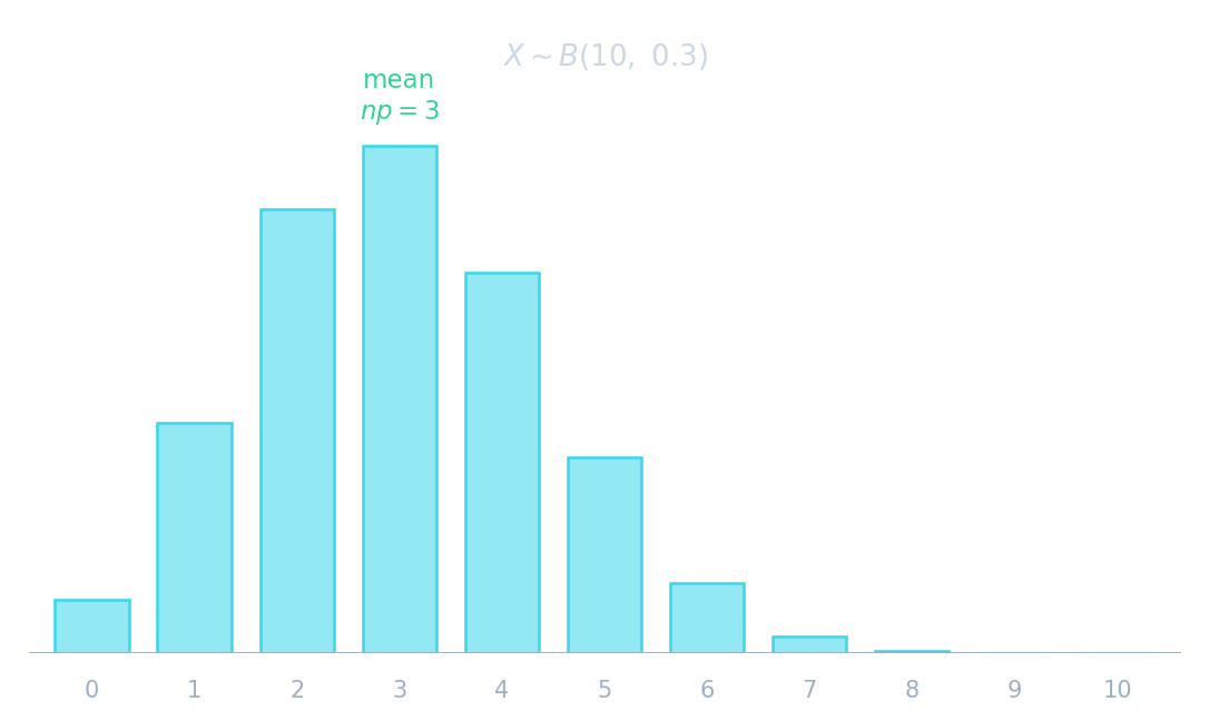
Each bar is P(X = r) for B(10, 0.3); the distribution peaks at the mean np = 3.
For X ~ B(10, 0.3), what is E(X) = np?
Difficulty 2/5 · 140 coins + a small bonus on first completion today
E(X) = np = 10 × 0.3 = 3.
For X ~ B(10, 0.3), what is Var(X) = np(1−p)?
Difficulty 2/5 · 140 coins + a small bonus on first completion today
Var(X) = np(1−p) = 10 × 0.3 × 0.7 = 2.1.
The geometric distribution 几何分布
- Geometric — the trial number of the first success:
- $P(X = r) = (1-p)^{r-1}p$
- $E(X) = \dfrac{1}{p}$.
For a geometric distribution with p = 0.2, E(X) = 1/p. Find it.
Difficulty 2/5 · 140 coins + a small bonus on first completion today
E(X) = 1/p = 1/0.2 = 5. On average, the first success occurs on trial 5.
Worked example — binomial
- $X \sim B(10, 0.3)$. Find $P(X = 2)$ and $E(X)$.
- $P(X = 2) = \dbinom{10}{2}(0.3)^2(0.7)^8 = 45 \times 0.09 \times 0.0576 = 0.233$.
- $E(X) = np = 10 \times 0.3 = 3$.
You've got it
- $E(X) = \sum x\,P(X=x)$; $\text{Var}(X) = \sum x^2 P(X=x) - (E(X))^2$
- binomial $B(n,p)$: $E = np$, $\text{Var} = np(1-p)$
- geometric: first success on trial $r$, $E = \dfrac1p$
Write from a binomial mean of 2
- A binomial distribution has n = 10 and p = 0.2.
- Find the mean and the variance.
For a binomial distribution with n = 10 and p = 0.2, what are the mean and the variance?
10 times 0.2 is 2. 2 times 0.8 is 1.6.
What is the mean?
Difficulty 1/5 · 100 coins + a small bonus on first completion today
np is 2 and np(1 - p) is 1.6.