This is the tenth course in University Electrical Engineering: control
systems 控制系统. EE06 gave you the system function. This course closes a
feedback 反馈 loop around it and answers the engineer's question: how do I
make the output follow the input quickly, accurately, and without ringing?
Units 10.1 and 10.2 build models of the plant 被控对象 (the thing being
controlled) and reduce them to one transfer function 传递函数.
Units 10.3 to 10.5 predict and shape the time response: specifications,
stability, root locus.
Units 10.6 and 10.7 work in the frequency domain: margins, Nyquist, PID and
compensators.
Unit 10.8 opens state space: models for many states, and a design method
built on linear algebra.
One habit runs through the whole course. Every design is checked in both
domains. A phase margin predicts a damping. A pole placement predicts an
overshoot. Every algebraic stability claim is confirmed by a second method:
Routh against the root locus, Nyquist against Routh. When two roads lead to
the same number, you can trust the number.
Why it matters. A cruise-control car holds 100 km/h on a hill. A 3D printer
places a droplet of plastic within 0.05 mm. Both start the same way: write
down what the physical system does, as an equation you can compute with.
The idea. Almost every physical domain stores, flows, and loses energy in
the same pattern. A hot tank stores heat, gains heat from a heater, and loses
heat to the room. A capacitor stores charge, gains it from a source, and leaks
it through a resistor. Written as one state variable 状态变量$x$, each of
them says
$$\text{(how fast } x \text{ changes)} \;=\; \text{(drive in)} \;-\; \text{(leakage out)}.$$
A first-order model has the form $\tau\, \dfrac{dx}{dt} + x = K\,u(t)$.
The Greek letter $\tau$ (tau) is the time constant 时间常数, measured in
seconds: it says how long the storage takes to respond. The symbol $K$ is the
DC gain: the final value of $x$ per unit of steady input $u$. With a step
input of size $U$, the solution is $x(t) = KU\,(1 - e^{-t/\tau})$, which
reaches 63.2% of its final value at one time constant.
Linearization 线性化. Real systems are not straight lines. A pendulum
obeys $\ddot\theta = -(g/l)\sin\theta$, which has no single gain. The fix is
to pick an operating point 工作点 (the state you work near) and replace
the curve by its slope there. Near rest, $\sin\theta \approx \theta$, so the
pendulum behaves like a spring with natural frequency 固有频率$\omega_n = \sqrt{g/l}$. For a swing of length $l = 0.9$ m, take $g = 9.81$
m/s² and get $\omega_n = \sqrt{9.81/0.9} = 3.30$ rad/s, about 0.53 Hz: a slow
playground swing. The same idea works for a tank draining at $q = 2\sqrt{h}$
(in m³/h with $h$ in m): the slope $\dfrac{dq}{dh} = 1/\sqrt{h}$ equals 0.5
near $h = 4$ m, and 1/3 near $h = 9$ m. The linear model is honest only near
its operating point, and the slope tells you how honest.
The armature-controlled DC motor: two physical laws, one inner feedback loop
Worked example 1: an RC circuit. Take $R = 2$ kΩ and $C = 100$ µF. The
resistor carries the current $\dfrac{v_{in} - v}{R}$ and the capacitor
integrates it, so
This is the first-order model with $\tau = RC = 2000 \times 100\times10^{-6} = 0.2$ s and $K = 1$. Step the input from 0 to 5 V and the capacitor reaches
$5(1 - e^{-1}) = 3.16$ V, which is 63.2%, after 0.2 s. Sense check: a bigger
$R$ or a bigger $C$ means a slower circuit, and the product $RC$ has units of
seconds, so the model is consistent.
Worked example 2: the armature-controlled DC motor. This model carries
through the whole course. The motor has rotor inertia $J = 0.01$ kg·m²,
friction $B = 0.1$ N·m·s, motor constant $K = 0.5$ (in N·m/A, numerically the
same as V·s/rad), and armature resistance $R = 1$ Ω. The inductance is small,
so we neglect it. Two physical laws couple the electrical and mechanical
sides:
Torque law: current makes torque, $T = K\,i$, with $T$ in N·m and $i$ in A.
Newton's law for the rotor: $J\,\dot\omega = T - B\,\omega$, where
$\omega$ is the shaft speed in rad/s.
The coupling runs both ways. The spinning armature also generates a back-EMF 反电动势
voltage $K\omega$, so Kirchhoff's voltage law (KVL) gives $V = R\,i + K\omega$. In the s-domain, with zero initial conditions, the two laws become
The model has one pole at $s = -35$ rad/s. The time constant is
$1/35 = 28.6$ ms: fast. The DC gain is $50/35 = 1.43$ rad/s of final speed
per volt. Sense check at DC: with everything constant the motor equations are
pure algebra, and indeed $\dfrac{K}{BR + K^{2}} = \dfrac{0.5}{0.35} = 1.43$.
The whole transient came from three physical constants, and the back-EMF
appears in the diagram as a feedback loop the motor builds for free. The two
variables here, $i$ and $\omega$, are exactly the state variables that unit
10.8 formalises.
Common mistakes.
Dropping the back-EMF term $K\omega$ from KVL. The result looks simpler and
is badly wrong: $\dfrac{K}{(Js+B)R} = \dfrac{50}{s+10}$ predicts 5 rad/s per
volt instead of 1.43 and a time constant of 100 ms instead of 28.6 ms. The
back-EMF's built-in feedback is what makes the real motor fast.
Using a linearization far from its operating point. The tank slope is 0.5
at $h = 4$ m and 0.33 at $h = 9$ m; one slope cannot serve both.
Unit slips: $J$ in kg·m², $B$ in N·m·s, $\omega$ in rad/s. Check that the
motor constant has the same value in both laws.
Summary. Storage, flow, and dissipation give $\tau\dot x + x = Ku$. Pick
the operating point, take the slope, and the world becomes linear near it.
The motor model $50/(s+35)$ is our running example from here on.
Why it matters. A block diagram 方框图 is how engineers speak about systems: a
poster of a car's cruise control is a block diagram, not a page of equations.
The idea. The transfer function $G(s)$ is the ratio of output
to input in the s-domain, with zero initial conditions. When blocks are
connected, arithmetic replaces algebra:
Series (one block after the other): multiply, $G = G_1 G_2$.
Parallel (both blocks feed the same sum): add, $G = G_1 + G_2$.
Feedback: divide by the loop, $T = \dfrac{G}{1 + GH}$.
The feedback formula deserves its one-line derivation. The error is $e = r - H\,y$ and the output is $y = G\,e$. Combine them: $y = G(r - Hy)$, move the
$GH\,y$ term across, and $y(1 + GH) = Gr$. The equation
$$1 + GH = 0$$
is the characteristic equation 特征方程. Its roots are the closed-loop
poles, so it holds the whole stability story. Reduce inner loops first, and
keep the denominator visible at every step.
Reduce the inner loop first, multiply the series, close the outer loop last
Worked example 1: one loop, read like a second-order system. Put
$G_1 = \dfrac{1}{s+1}$ and $G_2 = \dfrac{1}{s+2}$ in series with gain $K = 6$,
under unity feedback ($H = 1$):
Now read the second-order parameters by matching against $s^{2} + 2\zeta\omega_n s + \omega_n^{2}$. Here $\omega_n = \sqrt{8} = 2.83$ rad/s and
the damping ratio 阻尼比$\zeta = \dfrac{3}{2 \times 2.83} = 0.530$. That
sits inside the standard design region $0.4 \le \zeta \le 0.7$, and unit 10.3
turns it into an overshoot of about 14%.
Worked example 2: nested loops. An inner loop $\dfrac{2}{s}$ with
feedback gain 0.5 sits in series with $\dfrac{1}{s+1}$, all inside a
unity-feedback outer loop. Step 1, collapse the inner loop:
Read it: $\omega_n = \sqrt{3} = 1.73$ rad/s and $\zeta = \dfrac{2}{2\times 1.73} = 0.577$. A tangled diagram became two numbers. For genuinely tangled
diagrams, Mason's gain rule does all of this in one formula: sum the forward
path gains, subtract the products of loops that do not touch. Reach for it
when block algebra genuinely tangles, not before; on simple diagrams the
three rules above are faster.
Common mistakes.
Closing a loop as $\dfrac{G}{1+G}$ when $H \ne 1$. The return path carries
$GH$, not $G$.
Losing a minus sign at a feedback summer. The error is $r - Hy$. If you add
instead, the characteristic equation becomes $1 - GH = 0$ and every
stability claim flips.
Reducing the outer loop first. It still works, but the algebra explodes;
inner first is the discipline.
Summary. Series multiplies, parallel adds, feedback divides by $1 + GH$,
and the denominator of the result is the characteristic equation. Inner
loops first.
Why it matters. When a drone maker promises “settles within half a
second, overshoots less than 10%”, those are time-domain numbers. This unit
is the dictionary that turns pole positions into those numbers.
The idea. The second-order prototype carries the vocabulary:
$$G(s) = \frac{\omega_n^{2}}{s^{2} + 2\zeta\omega_n s + \omega_n^{2}}.$$
Its poles sit at $s = -\zeta\omega_n \pm j\,\omega_n\sqrt{1-\zeta^{2}}$. Read
the picture: the distance from the origin is $\omega_n$ (how fast), the
imaginary part rings, and the real part $-\zeta\omega_n$ decays. The damping
ratio is the cosine of the pole angle, so a ray from the origin at angle
$\arccos\zeta$ is a line of constant damping: one picture, one number.
One damping ratio, one shape: the whole family at $\omega_n = 4$ rad/s
The step response 阶跃响应 is the output when the input steps from 0 to 1.
With a unit step input, the standard results are
Here $M_p$ is the overshoot 超调量 (peak above the final value, as a
fraction), $t_p$ the peak time 峰值时间, and $t_s$ the settling time调节时间. The overshoot formula is not magic: the step response is
and the first peak comes where the derivative is zero, which lands at
$\omega_d t_p = \pi$; putting that back into the envelope gives $M_p$.
Steady-state error 稳态误差 needs one more idea. Count the integrators in
the open loop: that count is the system type 系统类型. A type-1 system (one
integrator) has zero steady-state error to a step, and its velocity error
constant 速度误差常数$K_v = \lim_{s\to0}\, sG(s)$ gives the ramp error
$\dfrac{1}{K_v}$. Read the constants off the loop before computing any
transient.
Worked example 1: one pair of numbers, four specifications. Take
$\omega_n = 4$ rad/s and $\zeta = 0.5$. Then $\omega_d = 3.46$ rad/s and the
poles are $-2 \pm j3.46$. Consistency check: the distance from the origin is
$\sqrt{2^{2} + 3.46^{2}} = 4 = \omega_n$, as it must be. The specifications:
The 10 to 90% rise time 上升时间 computes numerically from the step
response as 0.41 s. Sense check across domains: $\zeta = 0.5$ should come
with a phase margin near 50 degrees, and unit 10.6's working rule $\zeta \approx PM/100$ closes that loop.
Worked example 2: choose the gain to meet a damping spec. The plant is
$G = \dfrac{K}{s(s+2)}$ in unity feedback. The closed loop is
$\dfrac{K}{s^{2} + 2s + K}$, so matching the prototype gives $2\zeta\omega_n = 2$ and $\omega_n = \sqrt{K}$, hence $\zeta = 1/\sqrt{K}$. Demand
$\zeta = 0.45$:
Predict the response: $M_p = e^{-\pi(0.45)/0.893} = 0.205$, so 20.5%; peak
time $t_p = \dfrac{\pi}{2.22 \times 0.893} = 1.58$ s; settling $t_s \approx \dfrac{4}{0.45\times2.22} = 4.0$ s. Now the error constants, read off the
open loop: $K_v = \dfrac{4.94}{2} = 2.47$, so a unit ramp leaves a steady
error $\dfrac{1}{K_v} = 0.405$, while the step error is exactly zero because
the plant is type 1. Machine check: the simulated closed-loop step settles
to 1.000 and its first peak is 1.205.
Common mistakes.
Mixing $\omega_n$ with $\omega_d$. Peak time uses the damped frequency;
distance-from-origin uses $\omega_n$.
Quoting $t_s$ without its band. The 2% and 5% estimates differ by a factor
of $\tfrac{4}{3}$.
Applying second-order formulas to a system with zeros or extra poles
without checking that one pole pair really dominates.
Summary. Poles in, specifications out: $M_p$, $t_p$, $t_s$, and the error
constants. A damping ray on the pole plane is a constant-overshoot line.
Why it matters. Stability is the one property you must have before any
other design matters. A loop that rings itself into saturation is not badly
tuned; it is broken.
The idea. The closed loop is stable exactly when every root of the
characteristic polynomial has a negative real part. The Routh array 劳斯阵列
counts those roots without solving anything. Write the coefficients in two
rows, then fill downwards. Each new entry is a cross-multiply-and-divide of
the two rows above it, and the number of sign changes in the first column
equals the number of right-half-plane (RHP) roots. A first column with no
sign changes means no RHP roots: stable.
Worked example 1: count RHP roots. Test $s^{4} + 2s^{3} + 3s^{2} + 4s + 5$.
row
first column
second column
third column
$s^{4}$
1
3
5
$s^{3}$
2
4
0
$s^{2}$
$\tfrac{2\cdot3 - 1\cdot4}{2} = 1$
$\tfrac{2\cdot5 - 1\cdot0}{2} = 5$
$s^{1}$
$\tfrac{1\cdot4 - 2\cdot5}{1} = -6$
0
$s^{0}$
5
The first column reads $1,\, 2,\, 1,\, -6,\, 5$: two sign changes ($+1$ to
$-6$, then $-6$ to $+5$), so two RHP roots. Check by the exact roots, which
are $-1.29 \pm j0.86$ and $+0.29 \pm j1.42$: indeed two in the right half
plane, and the array said so without solving the quartic.
Worked example 2: find the gain range. For what $K$ is $s^{3} + 5s^{2} + 6s + K$ stable? Build the array:
Stability needs $\dfrac{30-K}{5} > 0$ and $K > 0$, so $0 < K < 30$. At
exactly $K = 30$ the $s^{1}$ row vanishes. That is not an error: a whole zero
row means symmetric roots, found from the auxiliary equation 辅助方程
built from the row above, $5s^{2} + 30 = 0$, so $s = \pm j2.45$. The system
sits on the boundary: marginal stability 临界稳定, a sustained oscillation
at 2.45 rad/s that neither grows nor dies. The next two units reach this same
boundary by two other roads.
The Routh test draws the stable design space before any root is solved
A design picture. For the family $s^{3} + as^{2} + 8s + K$, the same
cross-product gives the $s^{1}$ entry $\dfrac{8a - K}{a}$, so stability is
exactly $0 < K < 8a$: a straight boundary in the $(a, K)$ plane. The running
plant of this course, $s(s+2)(s+4)$, has $a = 6$ and limit $K = 48$: every
later unit lands on that same point.
Common mistakes.
Feeding the array an incomplete polynomial. The coefficients must cover
every power from $s^n$ down; a missing power gets coefficient 0.
Dividing a row by a negative number to simplify. Rescaling by a positive
number is free; a negative rescaling flips the very signs you are counting.
Treating a single zero in the first column as failure. Replace it with a
small positive $\varepsilon$ and continue; a whole zero row needs the
auxiliary equation.
Calling the $K = 30$ case “stable”. Poles on the axis mean marginal, not
stable: the oscillation never dies.
Summary. Build the array, count first-column sign changes, and the RHP
root count falls out with no root-finding. Parameter ranges read off one row.
Why it matters. Gain is the knob every amplifier, every controller, every
tuning session turns. The root locus tells you where the closed-loop poles go
as you turn it, before you build anything.
The idea. The root locus 根轨迹 is the set of points $s$ where the
angle condition holds for the loop $L(s) = K\,\dfrac{\prod(s-z_i)}{\prod (s-p_i)}$:
Each branch starts at an open-loop pole (at $K = 0$) and ends at a zero or at
infinity. The standard sketch rules all follow from that one condition:
Real-axis segments: a segment carries the locus when an odd number of
poles-plus-zeros lies to its right.
Asymptote 渐近线 angles $\dfrac{180°(2k+1)}{n-m}$, centred on the
centroid of the poles minus the zeros.
The breakaway point 分离点, where branches leave the real axis, solves
$\dfrac{d}{ds}\Bigl[\dfrac{\prod(s-p_i)}{\prod(s-z_i)}\Bigr] = 0$, and only
roots on the locus count.
The $j\omega$-axis crossing: put $s = j\omega$ into $1 + KL_0 = 0$ and
solve the real and imaginary parts.
Worked example 1: sketch the running plant. Take
$L = \dfrac{K}{s(s+2)(s+4)}$. Three poles at $0, -2, -4$ and no zeros, so $n - m = 3$ and the asymptotes leave the centroid $\dfrac{(0) + (-2) + (-4)}{3} = -2$ at $\pm 60°$ and $180°$. The real-axis locus is the segment
$[-2, 0]$ and the half-line $(-\infty, -4]$. The breakaway solves
giving $s = -0.845$ (on the locus: keep it) and $s = -3.155$ (between $-4$
and $-2$, off the locus: discard it). At the breakaway the gain is $K = |s(s+2)(s+4)| = 0.845 \times 1.155 \times 3.155 = 3.08$. The $j\omega$
crossing: with $s = j\omega$, the real part gives $K = 6\omega^{2}$ and the
imaginary part gives $\omega^{2} = 8$, so $\omega = 2.83$ rad/s and $K = 48$.
The same 48 that the Routh boundary drew.
Poles leave, meet at −0.845, bend to the asymptotes, and cross into instability at K = 48
Worked example 2: design for a damping spec on the locus. Require
$\zeta = 0.5$. The poles must sit on the ray at $\arccos 0.5 = 60°$ from the
negative real axis, that is on $s = -\sigma + j\,\sqrt{3}\,\sigma$ for some
$\sigma > 0$. Search along the ray for the point that satisfies the angle
condition. At $\sigma = 0.667$ the three pole angles are $120° + 40.9° + 19.1° = 180°$ exactly, so the design point is
Check the geometry: $|s^{*}| = \sqrt{0.667^{2} + 1.155^{2}} = 1.334$ and
$\dfrac{0.667}{1.334} = 0.500$, exactly the damping asked for. Check the
stability room: $K = 8.30$ sits far below the limit 48, so damping, not
stability, is what the $\zeta$-ray buys. The third pole at this gain sits at
$-4.67$, well to the left of the pair, which is why the pair dominates and
the second-order predictions hold.
Common mistakes.
Keeping an off-locus breakaway root. The quadratic gives two answers; only
points on the real-axis locus are physical.
Reading damping as distance from the origin. $\zeta$ is the cosine of the
pole angle: circles are constant $\omega_n$, rays are constant $\zeta$.
Assuming the asymptote crossing is the $j\omega$ crossing. Compute the
crossing from $1 + KL_0 = 0$; the asymptote is only a sketch aid.
Summary. Angle condition in, sketch out: segments, centroid, asymptotes,
breakaway, crossing. Design means walking the locus to a damping ray and
reading off the gain.
Why it matters. In industry you rarely know the exact pole positions; you
measure a frequency response. Margins are the engineering tolerance stated in
that language: how close to instability is this loop, in decibels and
degrees?
The idea. A Bode plot draws the loop gain $L(j\omega)$ as magnitude (in
dB, against log frequency) and phase (in degrees). Each pole contributes a
$-20$ dB/decade slope and up to $-90°$ of phase; each zero contributes the
opposite. Two numbers read off the plot carry the stability information:
Phase margin 相位裕度 PM: at the gain crossover 增益穿越 frequency
(where $|L| = 1$), how many degrees the phase sits above $-180°$.
Gain margin 幅值裕度 GM: at the phase crossover 相位穿越 (where
$\angle L = -180°$), the factor by which $|L|$ is below 1.
The working rule that ties the domains together is $\zeta \approx PM/100$: a
50° margin behaves like $\zeta \approx 0.5$, an overshoot near 16%. The
Nyquist criterion 奈奎斯特准则 makes stability counting exact. Plot
$L(j\omega)$ for $\omega$ from $-\infty$ to $+\infty$, count clockwise
encirclements 包围$N$ of the point $-1$, and the closed loop has $Z = N + P$
right-half-plane poles, where $P$ counts open-loop RHP poles. (A pole at the
origin, as in our running plant, is indented to the right on the Nyquist
contour; its infinite arc stays far from $-1$ and changes nothing here.)
Read PM at the gain crossover; the phase never reaches −180°, so GM is infinite
Worked example 1: margins by arithmetic. Take
$L = \dfrac{100}{s(s+10)}$. The gain crossover solves $|L| = 1$, that is
$\omega\sqrt{\omega^{2}+100} = 100$. Squaring gives $\omega^{4} + 100\omega^{2} - 10^{4} = 0$, so
The phase there is $-90° - \arctan(7.86/10) = -90° - 38.2° = -128.2°$, so the
phase margin is $PM = 180° - 128.2° = 51.8°$. The gain margin is infinite:
the phase only approaches $-180°$ asymptotically. Cross-check in the time
domain: the closed loop is $\dfrac{100}{s^{2} + 10s + 100}$, exactly the
prototype with $\omega_n = 10$ and $\zeta = 0.5$, an overshoot of 16.3%. The
rule $\zeta \approx PM/100$ predicted 0.52 against an exact 0.5: a working
estimate, not a theorem.
One curve shape; gain slides it through −1. At K = 96 it wraps twice around the point
Worked example 2: the running plant, three ways. Take
$L = \dfrac{20}{s(s+2)(s+4)}$, the $\zeta = 0.5$ design with the gain more
than doubled. The phase reaches $-180°$ where the imaginary part of
$s(s+2)(s+4)$ vanishes, at $\omega = \sqrt{8} = 2.83$ rad/s, and there
The gain crossover solves $\omega\sqrt{\omega^{2}+4}\sqrt{\omega^{2}+16} = 20$, giving $\omega_{c} = 1.73$ rad/s. The phase there is $-154.3°$, so $PM = 25.7°$. The rule predicts $\zeta \approx 0.26$ and a ringing response;
simulating the exact closed loop gives 48% overshoot, the behaviour the
margin promised. Now the Nyquist check. The magnitude at the $-180°$
frequency is $K/48$, so at $K = 20$ the curve passes 0.42 to the
right of $-1$: no encirclement, stable. At $K = 48$ it passes exactly through
$-1$: marginal. At $K = 96$ it wraps twice clockwise around $-1$, so $Z = N + P = 2 + 0 = 2$ closed-loop RHP poles. Routh on $s^{3} + 6s^{2} + 8s + K$
says unstable for $K > 48$, with two RHP roots at $K = 96$. Three methods,
one answer.
Common mistakes.
Reading margins off the closed-loop response. Margins live on the loop
gain $L$, before the loop closes.
Mixing up the two crossovers. PM belongs to the gain crossover; GM to the
phase crossover.
Counting encirclements of the origin. The criterion counts crossings of
the point $-1$, and with this sign convention clockwise is the positive
direction.
Forgetting $P$. If the plant itself has RHP poles, $Z = N + P$ needs that
count; $N$ alone is not the answer.
Summary. Bode gives PM and GM in seconds; $\zeta \approx PM/100$ carries
them into the time domain; Nyquist counts RHP poles exactly, and all three
must agree with Routh.
The proportional 比例 term reacts now. The integral 积分 term
remembers: it removes steady-state error by raising the system type. The
derivative 微分 term anticipates, adding damping proportional to how fast
the error moves. In the series (ideal) form, $u = K_{p}\bigl(e + \frac{1}{T_i}\int e\,dt + T_d\dot e\bigr)$, the tuning constants are the
integral time $T_i$ and the derivative time $T_d$, both in seconds.
The classical first cut is Ziegler-Nichols ultimate-gain tuning: raise the
proportional gain until the loop just oscillates, record the ultimate gain
$K_u$ and oscillation period $T_u$, and look up the row of the table. The
price list matters as much as the gains. P alone never removes steady-state
error. I adds phase lag. D amplifies measurement noise, and it must act on
the measured output rather than the reference, or every setpoint change
kicks the actuator.
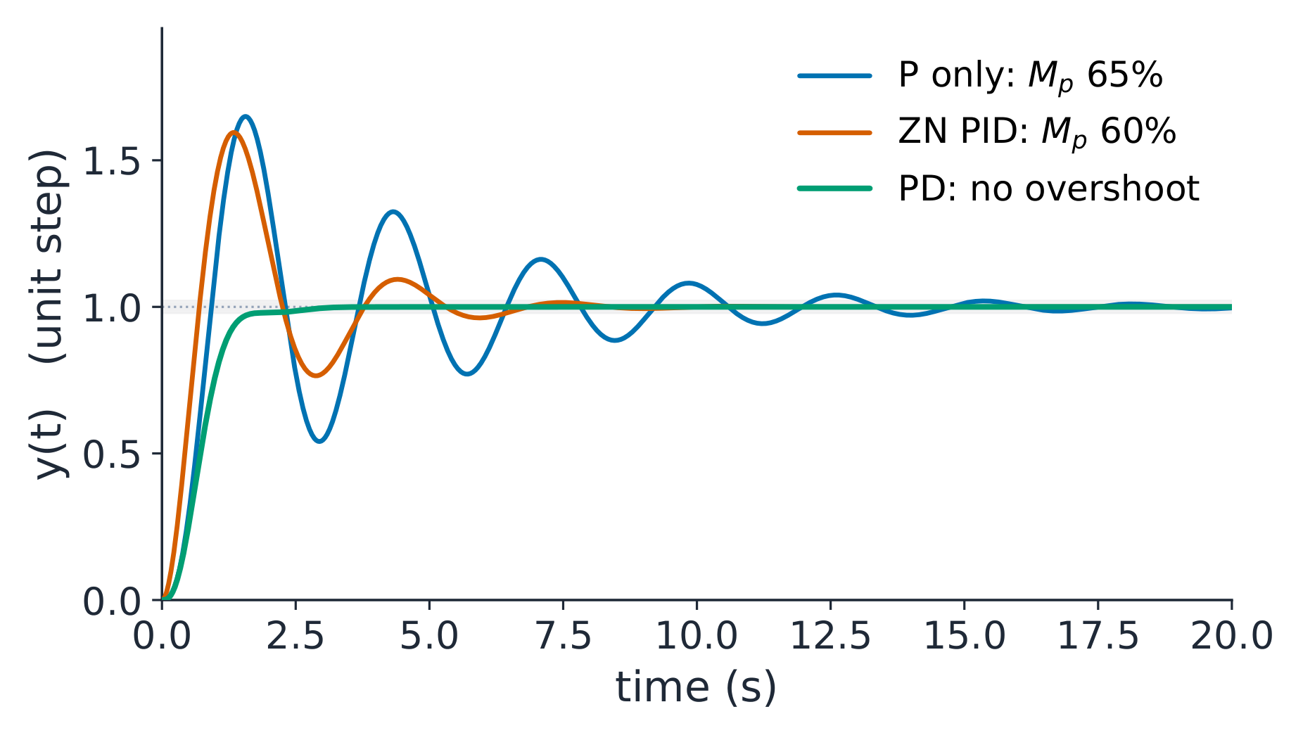
One plant, three tunings; every curve simulated from the closed-loop equations
Worked example 1: Ziegler-Nichols on the running plant. The loop
$\dfrac{K}{s(s+2)(s+4)}$ oscillates at $K_u = 48$ with $\omega_u = \sqrt{8} = 2.83$ rad/s (the Routh and Nyquist boundary), so the period is $T_u = \dfrac{2\pi}{2.83} = 2.22$ s. The PID row of the table gives
What do you actually get? With P alone at $K_p = 28.8$, the closed loop
$s^{3}+6s^{2}+8s+28.8$ has poles $-5.50$ and $-0.25 \pm j2.27$: 65%
overshoot, settling around 15 s, and a permanent ramp error
$\dfrac{1}{K_v} = \dfrac{8}{K_p} = 0.278$. The Ziegler-Nichols PID removes that error
completely, because the integrator raises the type, and its first overshoot
is 60%, decaying to about a sixth each cycle: the recipe aims at a
quarter-decay, not at comfort. The honest lesson: the table lands
you in the neighbourhood in one experiment, and it does not finish the job.
Worked example 2: finish with derivative, and size a lead. Keep $K_p = 28.8$ and add derivative. The PD loop's characteristic polynomial is
$s^{3} + 6s^{2} + (8 + K_{p}T_d)s + K_{p}$: the D term literally adds to the
damping coefficient. Raise $T_d$ from the Ziegler-Nichols value until the
ringing stops. At $T_d = 0.5$ s the polynomial is $s^{3}+6s^{2}+22.4s+28.8$
with poles $-2$ and $-2 \pm j3.22$. Where derivative acts matters: on the
measurement (the right practice, as below) the reference step meets no
zero, and the simulated step shows no overshoot at all, settling in 2.1 s.
On the error the PD zero at $-2$ cancels the real pole and the surviving
pair, $\zeta = 2/3.79 = 0.53$, still rings at about 14%: damping either way,
but only the measurement form is kick-free. The ramp error stays $0.278$:
derivative buys damping, not accuracy. For accuracy and speed together you
combine the terms and retune, which is exactly the exercise on sheet 10.7.
When the plant has no clean ultimate gain, frequency-domain lead
compensation does the same job. A lead compensator 超前校正装置$\dfrac{1+\tau s}{1+\alpha\tau s}$ with $0 < \alpha < 1$ puts a zero below a
pole and buys phase at one frequency. The maximum lift is
For a +45° lift, $\alpha = \dfrac{1-\sin 45°}{1+\sin 45°} = 0.172$. The same
network also lifts the high-frequency gain by $\dfrac{1}{\alpha} = 5.8$,
which the design must then absorb, usually by lowering the main gain. A lag
network is the same pair with $\alpha > 1$: it buys low-frequency gain for
error reduction, at the price of phase lag.
Anti-windup 抗饱和 belongs in every real implementation. When the
actuator saturates, the integrator keeps accumulating error it cannot spend,
and on recovery it dumps the stored action as one large overshoot. The two
standard cures: clamp the integrator while the output saturates, or
back-calculate, feeding a gain times the saturation excess back to reduce
the integral. Without one of these, the first real saturation eats every
margin you designed.
Common mistakes.
Running the ultimate-gain method on a plant that never oscillates. A
first-order or heavily damped plant has no $K_u$; use the step-response
variant of the table instead.
Taking derivative of the error instead of the measurement. A setpoint step
has an infinite slope, and the D term kicks the actuator.
Confusing the tuning forms. The series constants $K_p, T_i, T_d$ are not
the parallel gains: $K_i = K_p/T_i$ and $K_d = K_p T_d$.
Designing a lead network and forgetting its $\dfrac{1}{\alpha}$
high-frequency gain lift, which erodes the very margin you bought.
Summary. P reacts, I remembers, D anticipates; each buys one behaviour
and charges a known price. Use the table for the first cut, margins for the
refinement, and anti-windup for reality. The interactive lab on the course
page lets you turn exactly these two knobs, gain and damping, and watch
overshoot, settling and stability move.
Explore
One knob for gain, one for damping
Move the gain Kp and the derivative time Td and watch overshoot, settling and stability change together; gain alone breaks the loop at Kp = 48, and damping repairs it.
Why it matters. Transfer functions describe one input and one output.
Modern controllers, like a balancing robot or a drone running four loops at
once, live on state space, where several internal variables are modelled and
fed back together.
The idea.State space 状态空间 writes the system as $n$ first-order
equations instead of one $n$-th-order polynomial:
$$\dot{x} = Ax + Bu,
\qquad
y = Cx + Du,$$
where $x$ is the state vector, $u$ the input, $y$ the measured output, and
$A$, $B$, $C$, $D$ are matrices of constants. Intuition: the states are $n$
drawers of memory. The matrix $A$ says how each drawer pushes the others,
$B$ says where the input enters, and $C$ says what you measure. The
eigenvalues 特征值 of $A$ are the poles of the system, because
$\det(sI - A) = 0$
is exactly the characteristic equation. With zero input, the solution is
$x(t) = \Phi(t)\,x(0)$, where the transition matrix 状态转移矩阵$\Phi(t) = e^{At}$ is the matrix exponential, computed as the infinite
series $I + At + \dfrac{(At)^{2}}{2!} + \cdots$, which converges for every
square matrix.
Trajectories straighten onto the slow eigenvector: the tail of every response is the slow pole
Worked example 1: read a model, verify its decay. Take
$G(s) = \dfrac{8}{(s+2)(s+4)} = \dfrac{8}{s^{2}+6s+8}$. In companion form,
The DC gain checks the construction: $-CA^{-1}B = \tfrac{8}{8} = 1$,
matching the plant gain at $s = 0$. The eigenvalues of $A$ are $-2$ and
$-4$, exactly the poles. Now the transition matrix at $t = 0.5$ s, evaluated
by the series:
Its eigenvalues are $e^{-1} = 0.368$ and $e^{-2} = 0.135$: each pole becomes
its own decay factor per half-second. That is the deep identity: the matrix
exponential is the pole, made real. Starting from $x(0) = [1,\;0]^{T}$, the
state after 0.5 s is the first column, $[0.600,\; -0.930]^{T}$. In the
phase plane every trajectory straightens onto the slow eigenvector $[1, -2]^{T}$, which is why the $\lambda = -2$ pole owns the tail of the
response.
Worked example 2: pole placement by linear algebra. With full-state
feedback $u = -K_{fb}\,x$ (here $K_{fb}$ is a row vector of gains, not the
loop gain), the closed-loop matrix is $A - BK_{fb}$ and you choose its
characteristic polynomial directly. Demand both poles at $-10$, that is
$s^{2} + 20s + 100$. With $B = [0,\;1]^{T}$ and $K_{fb} = [k_1,\; k_2]$,
whose characteristic polynomial is $s^{2} + (6+k_2)s + (8+k_1)$. Match
coefficients: $k_1 = 92$ and $k_2 = 14$. The check is one line: the
eigenvalues of $A - BK_{fb}$ compute to $-10$ and $-10$ exactly. What the
root-locus unit did by searching along a ray, state feedback does by solving
linear equations, and it can place poles that no cascade of compensators
reaches, provided the input can actually drive every state direction. That
property is controllability 能控性, checked by the rank of the matrix
$[\,B\;\;AB\;\;\cdots\,]$, which is 2 here, so both poles are placeable.
When the states are not measured, an observer estimates them; that is the
door to the next course.
Common mistakes.
Forgetting $C$. The states are not the output; the transfer function is
$C(sI-A)^{-1}B + D$, and dropping $C$ quietly changes the DC gain.
Taking $e^{At}$ element by element. The matrix exponential is defined by
the series, and its off-diagonal entries are not exponentials of the
entries.
Assuming pole placement always works. If $[\,B\;\;AB\;\;\cdots\,]$ loses
rank, some directions are unreachable and no $K_{fb}$ exists; check
controllability first.
Mixing conventions. This course uses column states and a row $K_{fb}$; a
textbook with row states flips every product.
Summary.$A$ holds the dynamics, its eigenvalues are the poles, $e^{At}$
is the free response, and $u = -K_{fb}x$ turns design into linear algebra,
guaranteed by controllability.