This topic studies consumers, costs and firms in more detail. Start by comparing choices inside a budget, not by assuming that buying more always gives more satisfaction.
The price system and the microeconomy (A Level)
A-Level Economics · Topic 7
 18:50
18:50
The price system and the microeconomy (A Level)
Look at these shoppers. Each has a limited budget, and every extra thing they buy gives a little less pleasure than the last. Now a huge steel plant: it makes…
English narration · English + 中文 subtitles burned in
7.1
Utility and consumer choice

Syllabus
- explain total and marginal utility and the law of diminishing marginal utility
- derive the equi-marginal principle and explain how it relates to the demand curve, including the limitations of the marginal utility approach
Source: Cambridge International syllabus
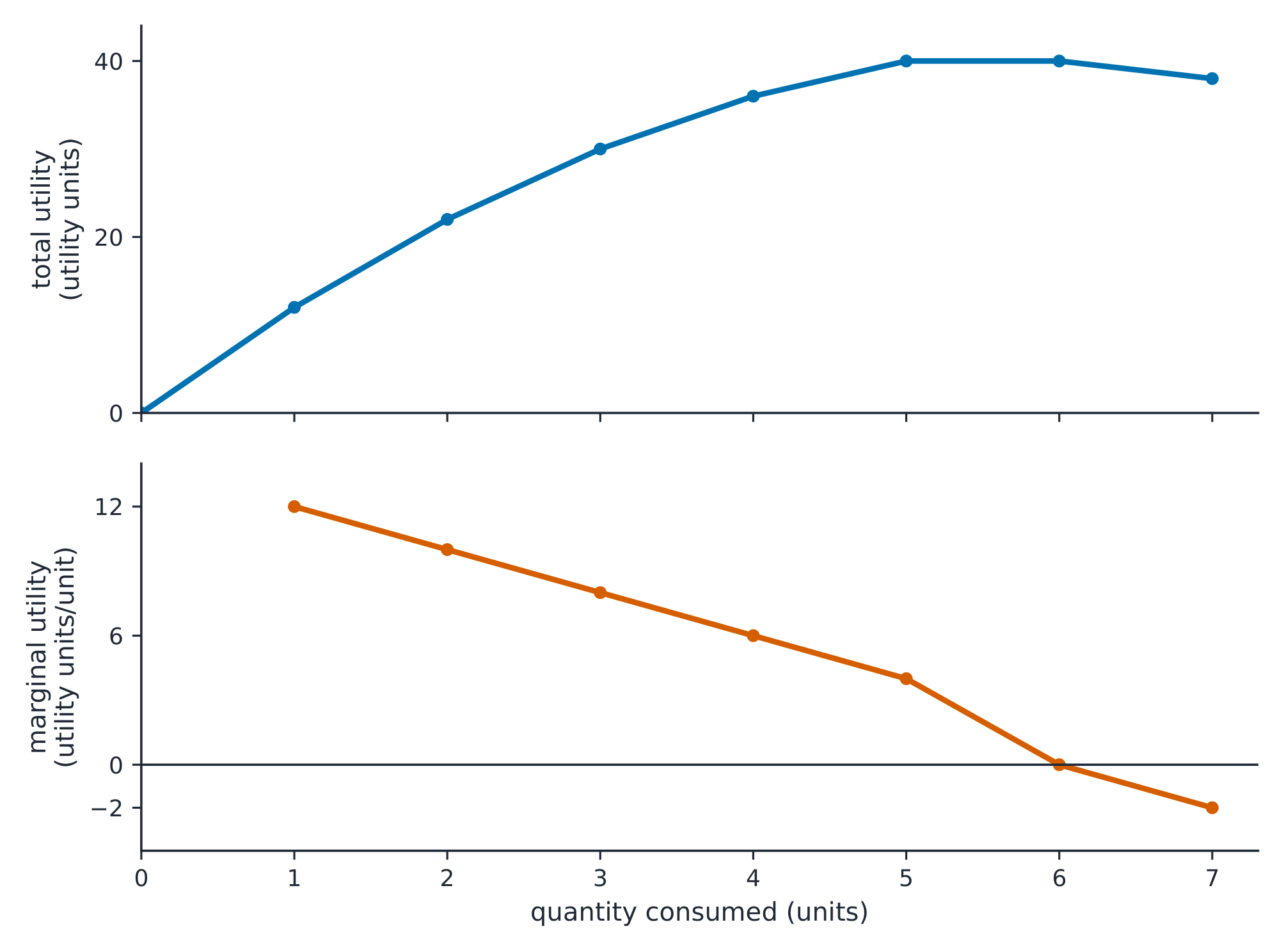
utility 效用 means satisfaction. The numbers below are illustrative utility units for one person. They are a model, not objective measurements that can be compared across people.
Calculate total and marginal utility
total utility 总效用 is satisfaction from the whole quantity consumed. marginal utility 边际效用 is the change in satisfaction from an extra unit. With other influences unchanged, diminishing marginal utility 边际效用递减 means each extra unit gives less additional satisfaction.
| Quantity | TU | MU of extra unit |
|---|---|---|
| 0 | 0 | — |
| 1 | 12 | 12 |
| 2 | 22 | 10 |
| 3 | 30 | 8 |
| 4 | 36 | 6 |
| 5 | 40 | 4 |
| 6 | 40 | 0 |
| 7 | 38 | −2 |
Worked example. MU is a change, not TU divided by quantity. For one-unit steps:
$$MU=\frac{\Delta TU}{\Delta Q}.$$
$$MU_4=\frac{TU_4-TU_3}{4-3}=\frac{36-30}{1}=6\text{ utility units/unit}.$$
$$MU_6=\frac{TU_6-TU_5}{6-5}=\frac{40-40}{1}=0.$$
$$MU_7=\frac{TU_7-TU_6}{7-6}=\frac{38-40}{1}=-2\text{ utility units/unit}.$$
TU rises while MU is positive, stays unchanged for the zero-MU sixth unit, and falls for the negative-MU seventh unit. Diminishing MU does not itself imply that TU always rises. Here TU reaches 40 at both 5 and 6 units.
Compare all feasible bundles
Income is £8; A costs £2/unit and B £1/unit. Only whole units can be bought, with at most 4A and 8B available. Assume the utilities of A and B add without interaction. A's MU for units 1–4 is 12, 8, 4, 0. B's MU for units 1–8 is 7, 6, 5, 4, 3, 2, 1, 0. Add successive MU values to calculate each good's TU.
For example, 2A gives $12+8=20$ utility and 4B gives $7+6+5+4=22$. The budget and combined-utility relationships are:
$$I=P_AQ_A+P_BQ_B.$$
$$I=P_AQ_A+P_BQ_B=\text{\pounds}2/\text{unit}\times2\text{ units}+\text{\pounds}1/\text{unit}\times4\text{ units}=\text{\pounds}8.$$
$$TU=TU_A(Q_A)+TU_B(Q_B).$$
$$TU(2,4)=TU_A(2)+TU_B(4)=20+22=42.$$
Since all additional utility in the available ranges is non-negative, a best bundle can be found among the whole-unit bundles that spend the full budget:
| A units | B units | Spending | Combined TU |
|---|---|---|---|
| 0 | 8 | £8 | 28 |
| 1 | 6 | £8 | 39 |
| 2 | 4 | £8 | 42 |
| 3 | 2 | £8 | 37 |
| 4 | 0 | £8 | 24 |
The best listed bundle is 2A and 4B. A high first-unit MU alone does not identify the best complete budget allocation.
The equi-marginal principle and its conditions
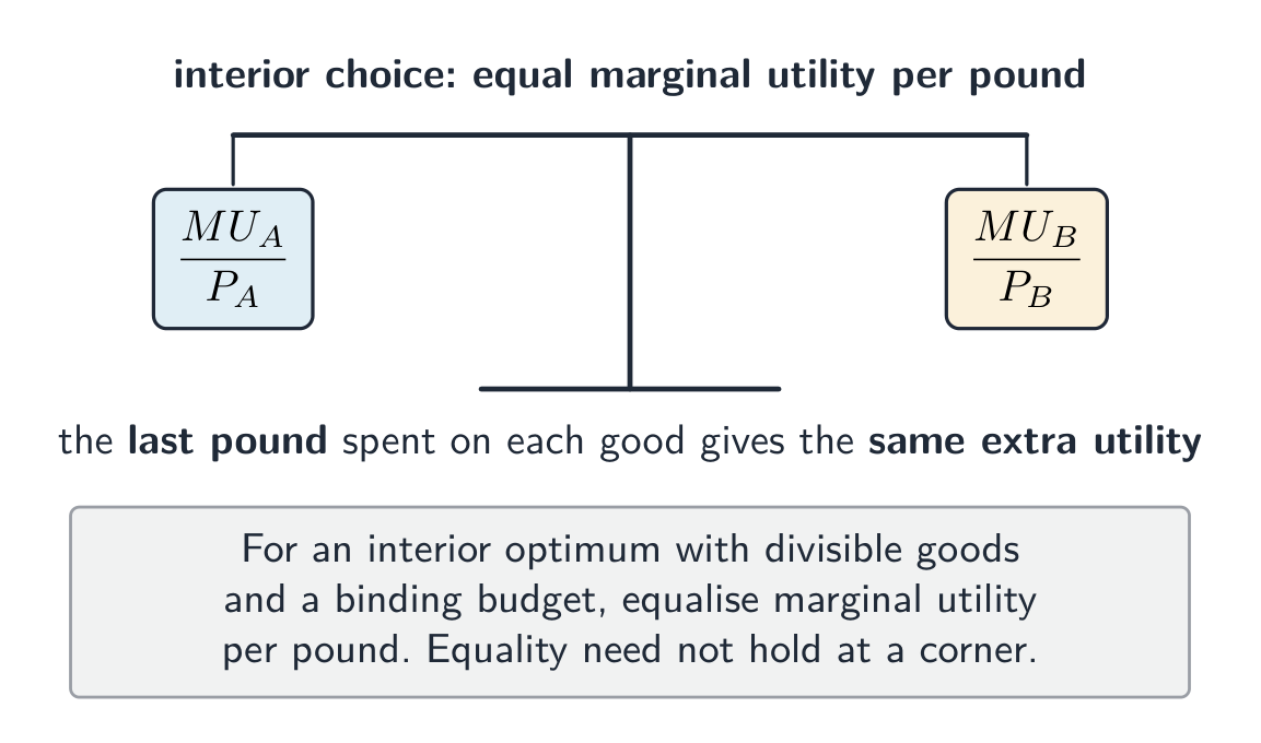
The equi-marginal principle 等边际原则 compares extra utility per pound spent. For a usual interior optimum with divisible goods and a binding budget, the ratios are equal:
$$\frac{MU_A}{P_A}=\frac{MU_B}{P_B}.$$
At the chosen 2A/4B bundle, the last A unit gives 8 utility and the last B unit gives 4:
$$\frac{MU_A}{P_A}=\frac{8\text{ utility units/unit}}{\text{\pounds}2/\text{unit}}=4\text{ utility units/\pounds}.$$
$$\frac{MU_B}{P_B}=\frac{4\text{ utility units/unit}}{\text{\pounds}1/\text{unit}}=4\text{ utility units/\pounds}.$$
Compare MU per pound, not MU alone. If a small transfer of spending can buy more extra utility from A than it gives up from B, reallocating can improve satisfaction. At a corner or with indivisible goods, exact equality may not be possible. Check feasible bundles and the budget instead of forcing the equation to hold.
A change in tastes: recheck the optimum
Keep prices and income unchanged but double every MU value for B, leaving A unchanged. Combined utility at each full-budget bundle becomes:
| A units | B units | New TU |
|---|---|---|
| 0 | 8 | 56 |
| 1 | 6 | 66 |
| 2 | 4 | 64 |
| 3 | 2 | 50 |
| 4 | 0 | 24 |
The best listed bundle becomes 1A/6B: more B and less A, with the same £8 budget. Quantity can change because preferences change. A price fall is not the only reason someone might buy more.
Derive a demand response with other influences fixed
Return to the original preferences, keep income £8 and B's price £1, then cut A's price from £2 to £1. Within the same available quantities, the new full-budget comparisons are:
| A units | B units | TU with original tastes |
|---|---|---|
| 0 | 8 | 28 |
| 1 | 7 | 40 |
| 2 | 6 | 47 |
| 3 | 5 | 49 |
| 4 | 4 | 46 |
A's chosen quantity rises from 2 to 3 as its own price falls from £2 to £1: two points on this person's demand curve 需求曲线. The optimum is found by comparison even though exact MU/P equality is unavailable for this whole-unit choice. Holding preferences, income and the other price fixed is essential when deriving an own-price response.
Limitations of marginal-utility reasoning
The result is conditional on the person's preferences, budget and available goods. The tables also assume utility from A and B can be added without interaction. Utility numbers are illustrative rather than objective readings of satisfaction. Real choices may involve habits, incomplete information and changing preferences, and people need not explicitly calculate a table. The model gives a conditional prediction, not a universal instruction to buy 2A and 4B.
Explore
Diminishing marginal utility lab
total utility rises more slowly as quantity increases
Add units consumed and see why extra satisfaction usually falls.
Vocabulary
Train
| English |
|---|
| utility/juːˈtɪlɪti/ |
| total utility/ˈtəʊtl juːˈtɪlɪti/ |
| marginal utility/ˈmɑːdʒɪnl juːˈtɪlɪti/ |
| diminishing marginal utility/dɪˈmɪnɪʃɪŋ ˈmɑːdʒɪnl juːˈtɪlɪti/ |
| equi-marginal principle/ˈekwi ˈmɑːdʒɪnl ˈprɪnsɪpl/ |
| demand curve/dɪˈmænd kɜːv/ |
7.2
Indifference curves and budget lines
Syllabus
- explain indifference curves and budget lines and consumer equilibrium
- explain income and substitution effects for normal, inferior and Giffen goods
Source: Cambridge International syllabus
Calculate the affordable set
A budget line 预算线 shows bundles that use all income at the stated prices. Points below it are affordable; points above it are not. For divisible goods X and Y, spending cannot exceed income:
$$P_XQ_X+P_YQ_Y\le I.$$
On the line, equality holds. With X horizontal, rearrange to express Y:
$$Q_Y=\frac{I}{P_Y}-\frac{P_X}{P_Y}Q_X.$$
The vertical intercept is $I/P_Y$, the horizontal intercept is $I/P_X$, and the slope is $-P_X/P_Y$.
Worked example. Income is £24; X costs £4/unit and Y costs £1/unit. Find the intercepts and check the bundle (3X,12Y).
$$Q_X^{\max}=\frac{I}{P_X}=\frac{\text{\pounds}24}{\text{\pounds}4/\text{unit}}=6\text{ units}.$$
$$Q_Y^{\max}=\frac{I}{P_Y}=\frac{\text{\pounds}24}{\text{\pounds}1/\text{unit}}=24\text{ units}.$$
$$E=P_XQ_X+P_YQ_Y=\text{\pounds}4/\text{unit}\times3\text{ units}+\text{\pounds}1/\text{unit}\times12\text{ units}=\text{\pounds}24.$$
The bundle uses the full budget. This establishes feasibility, not maximum satisfaction.
Income shifts and price pivots
Start from the same income and prices. Each change below occurs on its own; quantities are in units.
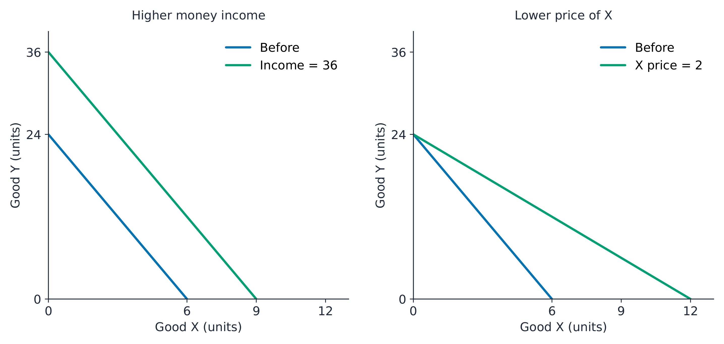
| Change | X intercept | Y intercept |
|---|---|---|
| Income rises to £36 | 9 | 36 |
| X price falls to £2/unit | 12 | 24 |
| Y price rises to £2/unit | 6 | 12 |
Higher money income moves both intercepts out in the same proportion, leaving the slope unchanged. Lower income shifts the line inward. A change in only X's price pivots the line about the unchanged Y intercept; a lower X price makes it flatter. A change in only Y's price keeps the X intercept fixed.
A parallel outward shift need not prove that money income rose. At unchanged £24 income, reducing both prices to two-thirds of their old levels also moves the intercepts from (6X,24Y) to (9X,36Y). The price ratio is unchanged. A taste change affects the preference map, not the budget line if income and prices stay fixed.
Rank satisfaction, then find the best affordable bundle
An indifference curve 无差异曲线 joins bundles giving the same satisfaction. An indifference map contains several such curves. In the usual model both goods are desirable: more of either, with the other unchanged, is preferred. Curves therefore slope downward; giving up one good requires more of the other to keep satisfaction unchanged. The usual bowed-in shape represents a declining willingness to give up Y for another X as X becomes more plentiful. Curves do not cross when preferences are consistent; a crossing would give contradictory rankings. These are model assumptions, not shapes required for every possible preference pattern.
Unlike the illustrative utility tables, this model needs only rankings of satisfaction, not an objective numerical measurement of it.
Worked example. In the illustrated map, (2X,18Y), (3X,12Y) and (6X,6Y) lie on the same curve. With prices £4/unit and £1/unit:
$$E=P_XQ_X+P_YQ_Y=\text{\pounds}4/\text{unit}\times2\text{ units}+\text{\pounds}1/\text{unit}\times18\text{ units}=\text{\pounds}26.$$
$$E=P_XQ_X+P_YQ_Y=\text{\pounds}4/\text{unit}\times3\text{ units}+\text{\pounds}1/\text{unit}\times12\text{ units}=\text{\pounds}24.$$
$$E=P_XQ_X+P_YQ_Y=\text{\pounds}4/\text{unit}\times6\text{ units}+\text{\pounds}1/\text{unit}\times6\text{ units}=\text{\pounds}30.$$
Equal satisfaction does not imply equal spending. Only (3,12) is affordable among these three bundles with £24 income.
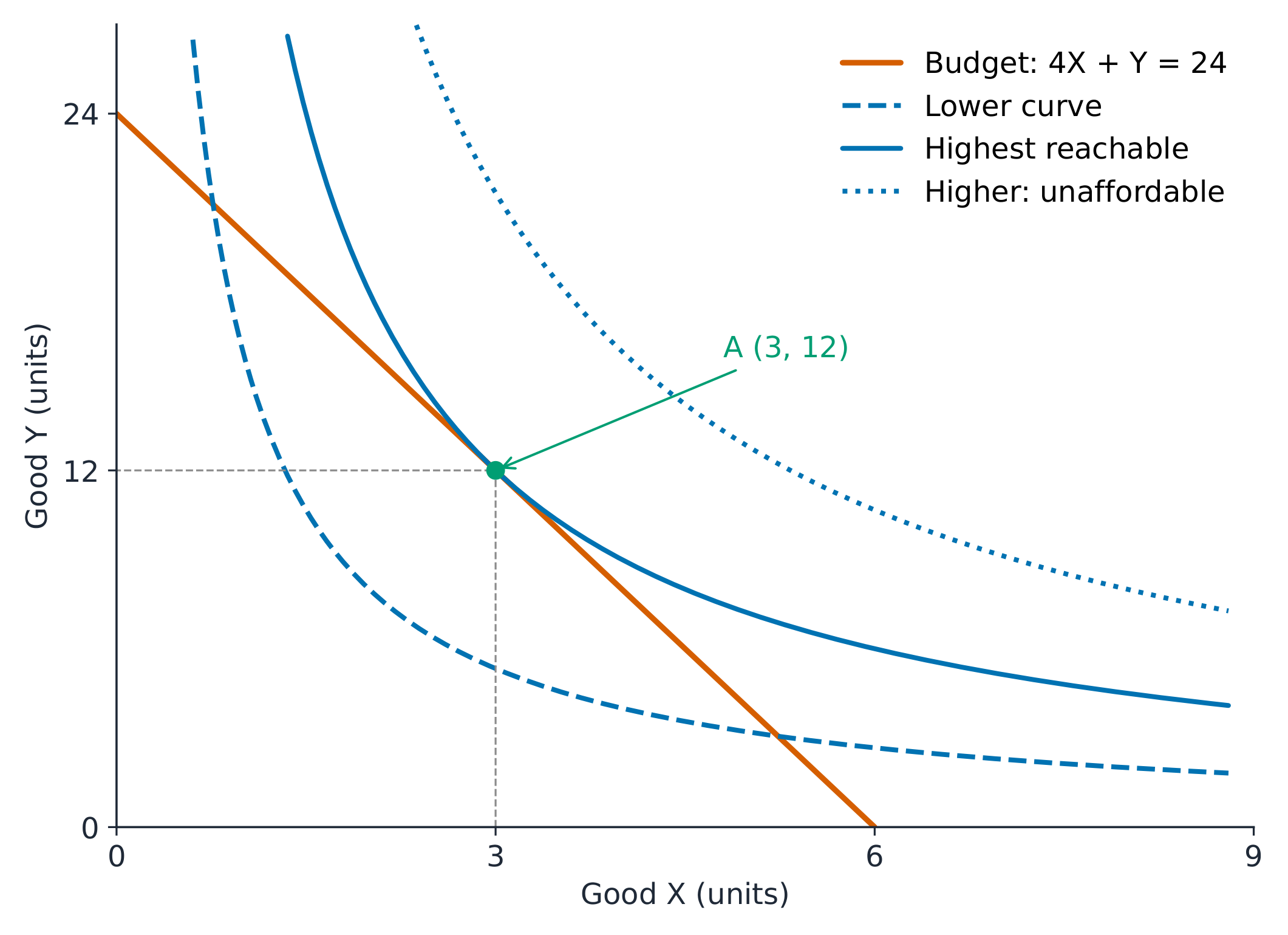
Consumer equilibrium 消费者均衡 is the most preferred affordable bundle. In this smooth example, the budget line is tangent to the highest reachable curve at A (3,12). A lower curve gives less satisfaction; a higher one has no affordable point.
Corner counterexample. Suppose preferences are represented by $U=3Q_X+Q_Y$, with £24 income and the same prices. The extra satisfaction per pound is:
$$\frac{MU_X}{P_X}=\frac{3\text{ utility units/unit}}{\text{\pounds}4/\text{unit}}=0.75\text{ utility units}/\text{\pounds}.$$
$$\frac{MU_Y}{P_Y}=\frac{1\text{ utility unit/unit}}{\text{\pounds}1/\text{unit}}=1\text{ utility unit}/\text{\pounds}.$$
Y gives more satisfaction per pound at every bundle. The best choice is 0X and 24Y, a corner. Its straight indifference curve is not tangent to the budget line. Divisible goods, smooth convex curves and an interior choice are extra conditions behind the familiar tangent diagram.
Separate income and substitution effects
A price fall changes relative prices and purchasing power. The substitution effect 替代效应 isolates the response to the changed price ratio while keeping satisfaction unchanged. The income effect 收入效应 then isolates the response to the gain in real purchasing power at the new price ratio. The total price effect is their sum. Money income need not change for real purchasing power to change.
In the following smooth illustrative map, income stays £24 and Y costs £1/unit. X's price falls from £4 to £1/unit. The old optimum is A (3X,12Y); the new optimum is B (12X,12Y).
Draw a comparison line parallel to the new budget line, touching the original indifference curve at C (6X,6Y). This compensated line has the new price ratio but reduces income enough to keep satisfaction unchanged. C is a comparison point, not the final choice with actual income.
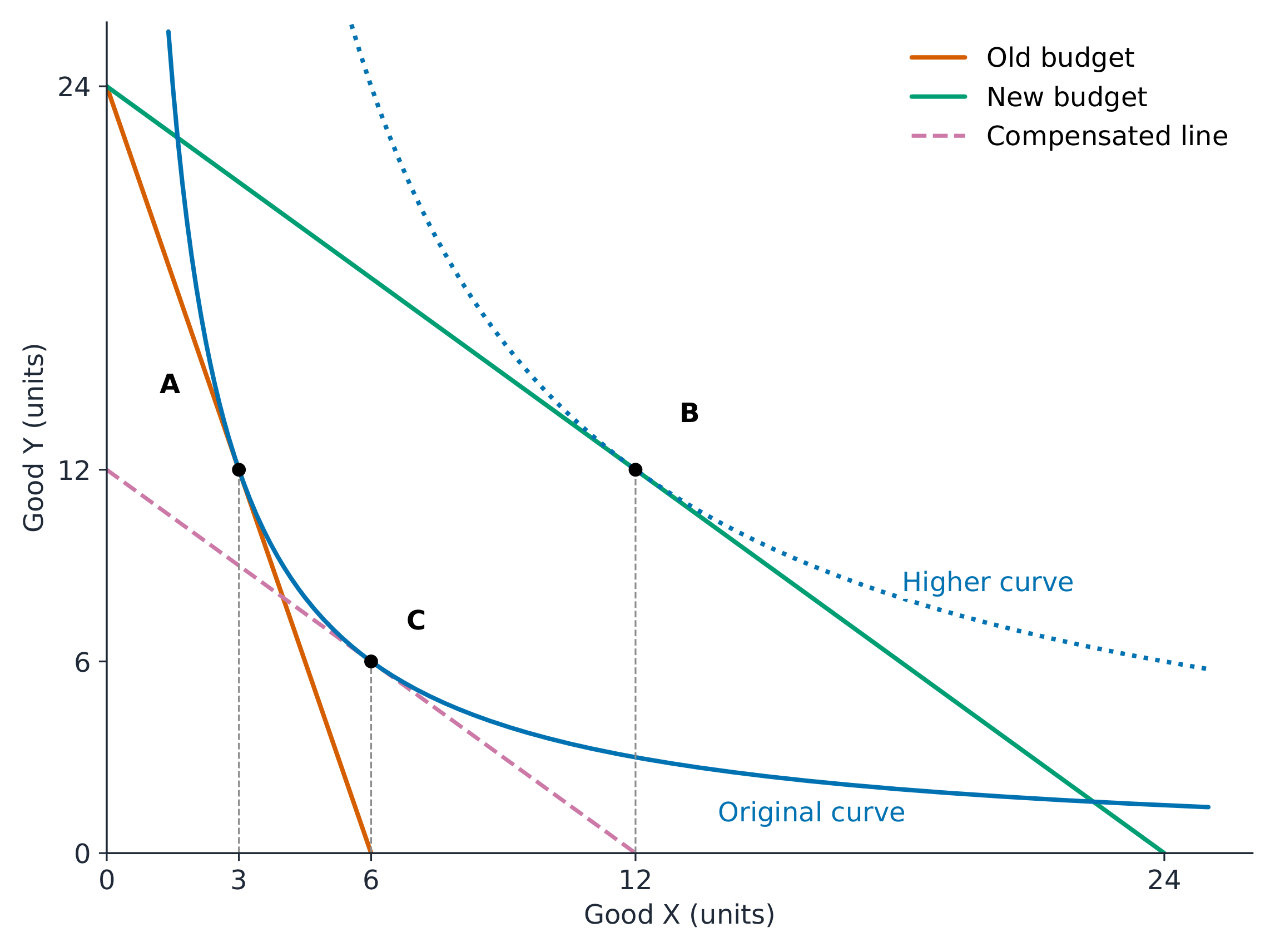
Worked example. Use the X coordinates to calculate each effect:
$$\Delta Q_X^{\rm sub}=Q_X^C-Q_X^A=6-3=+3\text{ units}.$$
$$\Delta Q_X^{\rm inc}=Q_X^B-Q_X^C=12-6=+6\text{ units}.$$
$$\Delta Q_X=\Delta Q_X^{\rm sub}+\Delta Q_X^{\rm inc}=3+6=+9\text{ units}.$$
This is a normal good 正常品 example: substitution and income effects both raise X. On the new-price comparison line C costs £12; restoring actual £24 income leads to B on a higher curve. The diagram is consistent with the stated coordinates and budgets; it is an illustration, not observed consumer data.
Inferior goods and the Giffen exception
For an inferior good 低档品, higher real income reduces the quantity chosen. The income effect opposes substitution towards the now cheaper good. If substitution is stronger, quantity still rises when price falls. A Giffen good 吉芬品 is the special inferior case where the opposing income effect is stronger, so quantity falls when its price falls, with other influences fixed. Inferiority alone does not establish Giffen behaviour.
These separate hypothetical price-fall cases are not extra points on the preceding map. All entries are changes in X quantity, in units.
| Case | Substitution | Income | Total |
|---|---|---|---|
| Normal | +3 | +6 | +9 |
| Inferior, not Giffen | +3 | −1 | +2 |
| Giffen | +3 | −5 | −2 |
The total follows from adding the two effects. Classify the inferior cases by the negative income effect; distinguish Giffen by its size relative to substitution. An upward-sloping own-price demand response requires the Giffen condition, not simply a cheap product or a low-income buyer.
Evaluate the model with the diagram
For an exam response about a price change, label both goods, show the budget pivot and the old/new highest reachable curves, then add the compensated line to distinguish the two effects. Compare normal, inferior and Giffen responses before judging the claim that a lower price always raises quantity. A pivot alone cannot prove that claim.
The model assumes consistent preferences, the ability to rank bundles and a choice of the most preferred affordable bundle. Two goods simplify the many alternatives available in real markets. Habits and incomplete information can affect choice; advertising or changing tastes can change the map itself. Indivisible goods or corner choices can prevent a smooth interior tangency. These limitations explain when a prediction may fail; simply listing them does not evaluate a particular price response.
Check yourself. Intercepts rise from (6X,24Y) to (9X,36Y). Give an income explanation and a price explanation. Then explain why a +3-unit substitution effect and a −5-unit income effect make a price fall reduce total quantity by 2 units.
Answer. At unchanged prices, income £24→£36 produces the shift; at unchanged £24 income, both prices falling to two-thirds of their old levels also does so. In the effects case, the good is inferior and the opposing income effect is larger, so it is Giffen over the illustrated change. The total price effect is $+3+(-5)=-2$ units.
Explore
Budget line lab
good B = income / priceB - slope x good A
Move quantity of one good and see the trade-off with the other good.
Vocabulary
Train
| English |
|---|
| indifference curve/ɪnˈdɪfrəns kɜːv/ |
| budget line/ˈbʌdʒɪt laɪn/ |
| consumer equilibrium/kənˈsuːmə ˌiːkwɪˈlɪbrɪəm/ |
| substitution effect/ˌsʌbstɪˈtjuːʃn ɪˈfekt/ |
| income effect/ˈɪŋkʌm ɪˈfekt/ |
| normal good/ˈnɔːml ɡʊd/ |
| inferior good/ɪnˈfɪərɪə ɡʊd/ |
| Giffen good/ˈdʒɪfən ɡʊd/ |
7.3
Efficiency and market failure

Syllabus
- explain productive and allocative efficiency, Pareto optimality and dynamic efficiency
- explain market failure, including from monopoly, externalities, public goods, information failure and factor immobility
Source: Cambridge International syllabus
Efficiency has several meanings. A plant can cut its cost per unit without making the right quantity for society, and a useful innovation can still leave someone worse off. State which test is being applied.
Productive efficiency: test cost per unit
Productive efficiency 生产效率 means producing at the lowest possible average cost 平均成本. Resources are used without avoidable waste. For a firm, compare its output with the minimum of the relevant average-cost curve; a large output alone does not establish efficiency.
Worked example. A plant has these illustrative monthly costs at unchanged input prices and product quality. Calculate average cost, then identify the lowest observed value.
| Output (units/month) | Total cost (£/month) | AC (£/unit) |
|---|---|---|
| 50 | 450 | 9 |
| 100 | 800 | 8 |
| 150 | 1350 | 9 |
$$AC=\frac{TC}{Q}=\frac{\text{\pounds}450/\text{month}}{50\text{ units/month}}=\text{\pounds}9/\text{unit}.$$
$$AC=\frac{TC}{Q}=\frac{\text{\pounds}800/\text{month}}{100\text{ units/month}}=\text{\pounds}8/\text{unit}.$$
$$AC=\frac{TC}{Q}=\frac{\text{\pounds}1350/\text{month}}{150\text{ units/month}}=\text{\pounds}9/\text{unit}.$$
100 units/month has the lowest AC among the observations. The full cost curve is needed to establish the overall minimum. Raising output from 100 to 150 lowers neither total cost nor average cost. A fall in input prices or product quality could also lower measured unit cost, so these must be controlled before inferring an improvement in the use of resources.
Allocative efficiency: compare the benefit and cost of extra output
Allocative efficiency 配置效率 means resources are allocated to the output mix that maximises net social benefit. The condition is marginal social benefit 边际社会收益 equal to marginal social cost 边际社会成本, with no remaining beneficial reallocation. If marginal benefit exceeds marginal cost 边际成本, a small expansion adds net benefit; if marginal cost exceeds marginal benefit, reduce output. The usual crossing with falling benefit and rising cost identifies the best quantity.
The familiar condition $P=MC$ applies when price represents consumers' marginal benefit and private benefits/costs match social ones. A price equal to private marginal cost does not prove allocative efficiency if external costs or benefits are ignored.
Worked example. In this separate continuous-output illustration, there are no external costs or benefits. MB means the benefit to consumers from extra output and MC its resource cost. Values are illustrative, not the cost data in the previous example.
| Output (units/month) | MB (£/unit) | MC (£/unit) | Direction |
|---|---|---|---|
| 3 | 9 | 5 | Expand |
| 5 | 7 | 7 | Best margin |
| 7 | 5 | 9 | Reduce |
At output near 3, extra output is worth more than it costs. Near 7, reducing output saves more cost than the benefit lost. At 5, the two margins are equal. This is a test of quantity and benefit, not a test of minimum average cost.

Productive and allocative efficiency need not occur at the same output. For example, the output where a demand curve meets marginal cost need not be at the minimum of average cost. Inspect each condition separately rather than treating low price, normal profit or high output as proof of both.
Pareto optimality: can someone gain without anyone losing?
A Pareto improvement makes at least one person better off and nobody worse off. Pareto optimality 帕累托最优 means no feasible Pareto improvement remains. It does not establish fairness or a unique best distribution.
Worked example. The following four outcomes are the complete feasible list in a toy model. A larger score means a better outcome for that person; the scores only rank outcomes and are not added across people.
| Outcome | Person 1 | Person 2 |
|---|---|---|
| A | 10 | 10 |
| B | 12 | 10 |
| C | 13 | 9 |
| D | 11 | 11 |
A→B helps Person 1 without harming Person 2; A→D helps both. A is therefore not Pareto optimal. B, C and D are each Pareto optimal within this complete feasible list: moving between them helps one person at the expense of the other. Their different distributions show why Pareto optimality alone does not select a fair outcome. If another feasible outcome were added, the judgement would need to be checked again.
Training or removing waste may create the resources for a Pareto improvement, but consider the training cost and who gains or loses. A rise in aggregate benefit is not by itself proof that nobody is worse off.
Dynamic efficiency: improvements over time
Dynamic efficiency 动态效率 concerns improvements through innovation, better methods and better products over time. It changes future production or consumption possibilities. Productive and allocative efficiency test the use and allocation of resources at a particular time.
Worked example. Successful research creates a process that makes the same 100 units/month, at unchanged product quality and input prices, for £600/month rather than £800/month:
$$AC_{\rm old}=\frac{TC_{\rm old}}{Q}=\frac{\text{\pounds}800/\text{month}}{100\text{ units/month}}=\text{\pounds}8/\text{unit}.$$
$$AC_{\rm new}=\frac{TC_{\rm new}}{Q}=\frac{\text{\pounds}600/\text{month}}{100\text{ units/month}}=\text{\pounds}6/\text{unit}.$$
This is evidence of an improvement in production possibilities. It does not prove the firm is at its new minimum AC, chooses the allocatively efficient output, passes the saving to consumers, or recovers the research cost. Those require further information. A new product or better quality can also be a dynamic improvement even when its unit cost does not fall.
Competition can encourage innovation by rewarding better quality or lower costs. Market power and profits may provide finance for a costly project, but they do not guarantee that it will be undertaken. Conversely, competition does not automatically prevent research or access to finance. Judge the incentive, available resources, ability to keep the gains from invention and actual results. Do not claim that a competitive firm cannot innovate simply because it earns normal profit in a long-run model.
Market failure: identify the mechanism and the allocation problem
Market failure 市场失灵 occurs when the market fails to allocate resources efficiently. A high price, unequal income or low profit is not sufficient evidence by itself. Identify the missing cost or benefit, the incentive problem or the constraint, and explain its effect on the quantity or use of resources.
Market power. A sole seller may restrict output even though buyers value extra output more than its full resource cost. Such mutually beneficial output is left unproduced. Compare benefit and cost at the margin; a high price alone does not prove this gap.
Externalities 外部性. A factory may ignore damage its smoke causes to nearby households. Its private calculation then understates the cost to society, potentially causing excess output. The next section distinguishes the production and consumption cases, including external benefits.
Public goods 公共物品 are non-rival and non-excludable. In a flood-warning broadcast, another listener does not reduce anyone else's reception and non-payers cannot be excluded from the signal. Residents can benefit while leaving others to pay, weakening voluntary private funding. The sum of benefits may justify provision even when a private seller cannot collect enough payment to cover cost. The allocation problem is possible underprovision, not an absence of value. Public ownership is not the definition; test rivalry and exclusion.
Information failure 信息失灵. If a buyer cannot assess a machine's safety, they may buy a model with hidden defects that they would reject with better information. Expected and informed benefits differ, potentially causing a poor allocation. The cost of acquiring information also matters.
Factor immobility 要素不流动性. Workers or capital may not move quickly to more useful activities despite higher returns. Retraining, relocation and other barriers delay adjustment. However, moving and training use real resources: unemployment or a price difference alone does not prove inefficiency. Explain why the barrier prevents a beneficial reallocation after allowing for those costs.
Check yourself. A process lowers unit resource cost from £8 to £6 at fixed quality and input prices. At the chosen output, marginal social benefit is £5/unit and marginal social cost £7/unit. A resident loses from the associated noise. Which efficiency claims follow?
Answer. The innovation is evidence of a dynamic improvement and lower cost at that output, but does not prove minimum AC. Because marginal social cost exceeds marginal social benefit at the chosen margin, reducing output would raise net social benefit: allocative efficiency has not been achieved. The resident's loss means the change is not a Pareto improvement as described, even if other people gain more in total.
Explore
Allocative efficiency
The market is allocatively efficient where supply meets demand — price equals marginal cost. Market failure pushes it away from that point.
Vocabulary
Train
| English |
|---|
| productive efficiency/prəˈdʌktɪv ɪˈfɪʃənsi/ |
| allocative efficiency/ˈæləkətɪv ɪˈfɪʃənsi/ |
| Pareto optimality/pæˈriːtəʊ ˌɒptɪˈmælɪti/ |
| dynamic efficiency/daɪˈnæmɪk ɪˈfɪʃənsi/ |
| market failure/ˈmɑːkɪt ˈfeɪlɪə/ |
| public good/ˈpʌblɪk ɡʊd/ |
| information failure/ˌɪnfəˈmeɪʃn ˈfeɪlɪə/ |
| factor immobility/ˈfæktə ɪˌməʊˈbɪlɪti/ |
| marginal social cost/ˈmɑːdʒɪnl ˈsəʊʃl kɒst/ |
| marginal social benefit/ˈmɑːdʒɪnl ˈsəʊʃl ˈbenɪfɪt/ |
| average cost/ˈævrɪdʒ kɒst/ |
| marginal cost/ˈmɑːdʒɪnl kɒst/ |
7.4
Externalities and social costs and benefits

Syllabus
- distinguish private, external and social costs and benefits
- analyse positive and negative externalities of production and consumption using marginal analysis and explain deadweight welfare loss
Source: Cambridge International syllabus
A factory's smoke may harm neighbours who did not choose its output. A vaccination may protect people other than the person receiving it. The private decision and its full effect on society can therefore differ. An externality is a cost or benefit affecting a third party outside the transaction, not simply any price paid by the buyer.
Calculate total private, external and social values
A private cost 私人成本 falls on the decision-maker; an external cost 外部成本 falls on third parties. The social cost 社会成本 includes both. A private benefit 私人收益 accrues to participants; an external benefit 外部收益 accrues to other people. The social benefit 社会收益 includes both.
Worked example: cost. A factory uses resources costing £800/month and causes pollution damage of £200/month. Assume these are all relevant costs for that output:
$$SC=PC+EC=\text{\pounds}800/\text{month}+\text{\pounds}200/\text{month}=\text{\pounds}1000/\text{month}.$$
The factory's private calculation omits the neighbours' damage. A compensation payment is a transfer between parties, not another resource cost to add on top of the same damage. Count each effect once; any separate administrative or prevention cost would need its own treatment.
Worked example: benefit. In a separate training programme, participants gain benefits valued at £1200/year and others gain £400/year as skills spread:
$$SB=PB+EB=\text{\pounds}1200/\text{year}+\text{\pounds}400/\text{year}=\text{\pounds}1600/\text{year}.$$
These are valuations of benefits, not just sales receipts. A price paid or received is not automatically the full benefit or resource cost to society. Use the same activity, quantity and time period when adding components.
Marginal values concern an extra unit
Marginal analysis 边际分析 compares changes. Marginal private cost 边际私人成本 (MPC) and marginal private benefit 边际私人收益 (MPB) concern the private cost and benefit of extra output or consumption. Marginal external cost 边际外部成本 (MEC) and marginal external benefit 边际外部收益 (MEB) concern its effects on third parties. MSC and MSB are the marginal social cost and benefit, defined in the efficiency section.
Worked example. An extra unit of production uses £7 of the firm's resources and imposes £2 of external damage:
$$MSC=MPC+MEC=\text{\pounds}7/\text{unit}+\text{\pounds}2/\text{unit}=\text{\pounds}9/\text{unit}.$$
In a separate service, an extra unit gives its user £5 of benefit and others £2:
$$MSB=MPB+MEB=\text{\pounds}5/\text{unit}+\text{\pounds}2/\text{unit}=\text{\pounds}7/\text{unit}.$$
These extra-unit values are not totals or averages. Dividing total social cost by quantity gives an average, not necessarily the marginal cost.
Use private and social equilibrium conditions separately
In the simple competitive-market model without corrective intervention, output is where $MPB=MPC$. The social test is $MSB=MSC$. With falling marginal benefit and rising marginal cost, the social intersection maximises net benefit. Monopoly, taxes or other distortions require separate treatment; the private intersection is not a universal rule for every market structure.
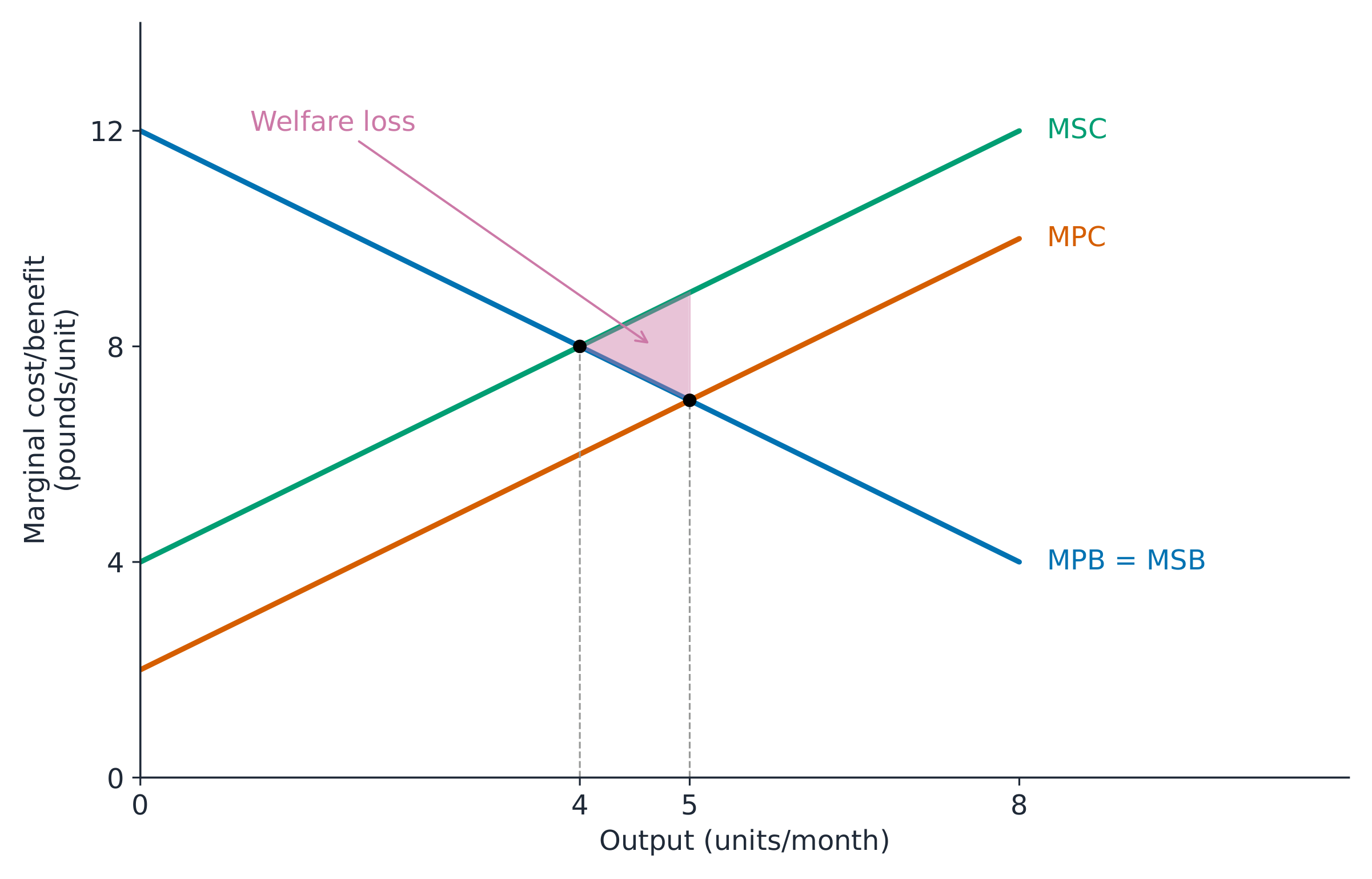
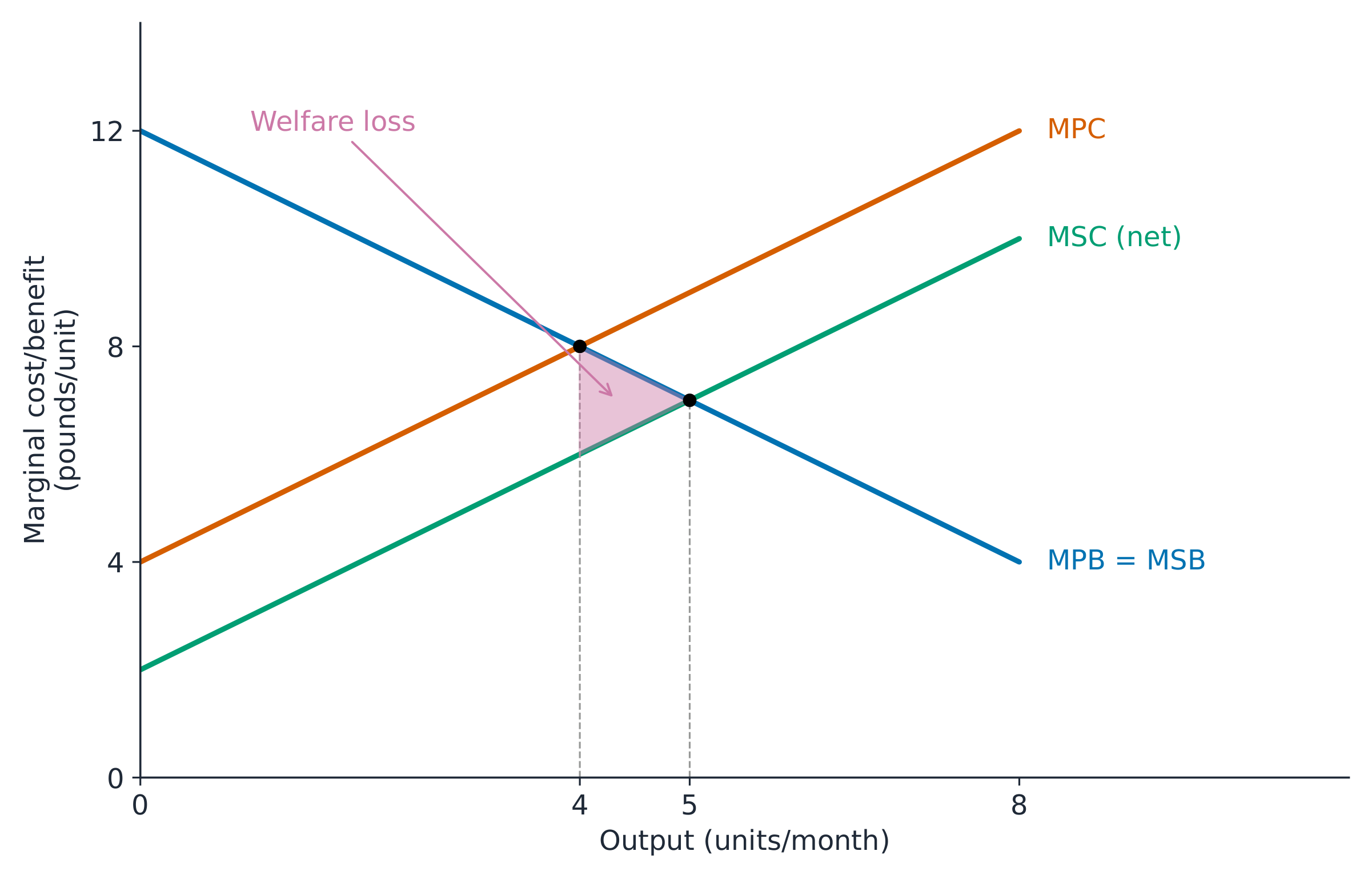
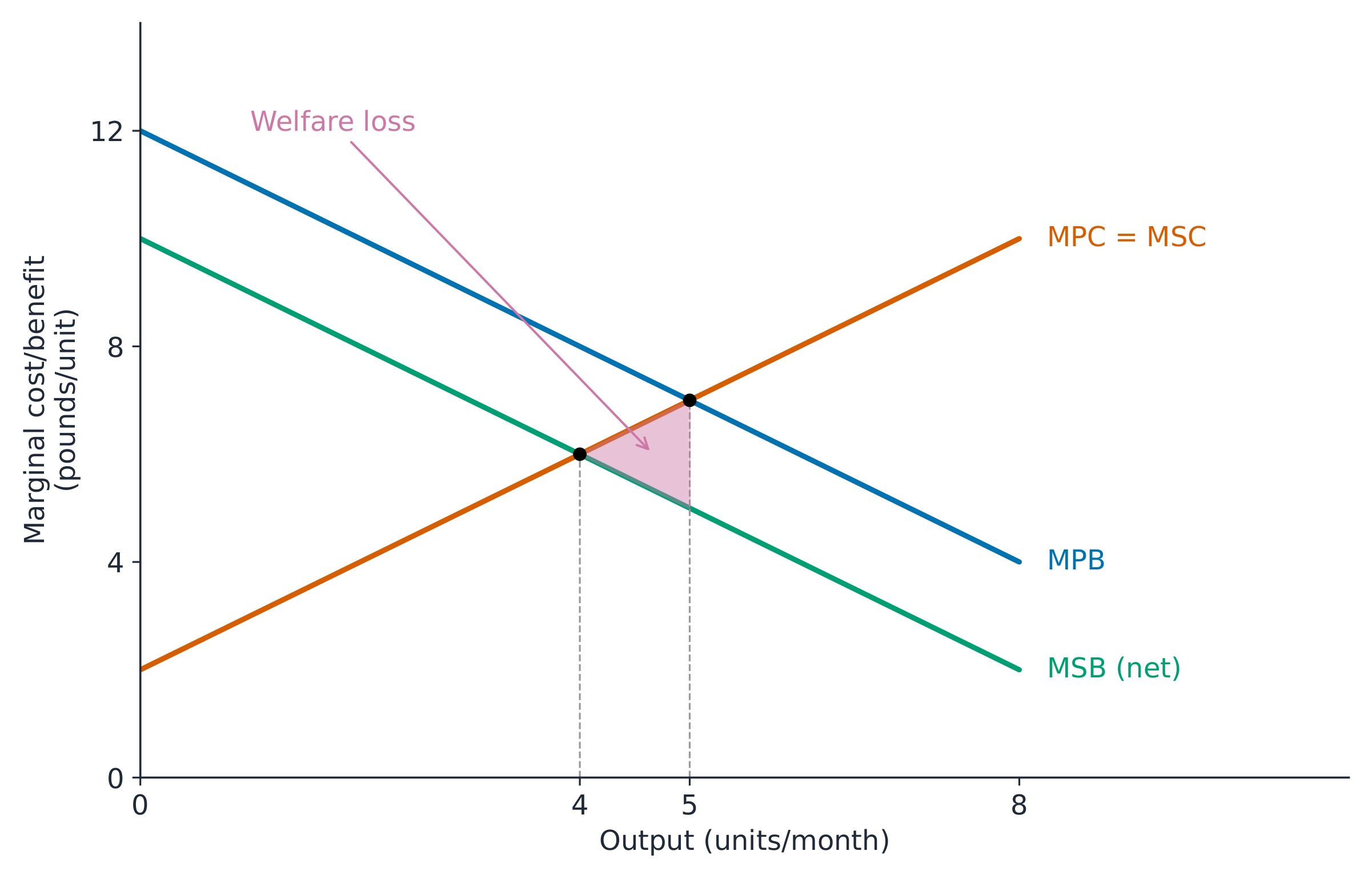
The following four diagrams are separate illustrations. Each isolates one spillover and assumes other distortions absent. A negative externality 负外部性 harms third parties; a positive externality 正外部性 benefits them. The diagram's cost/benefit convention must be stated so a spillover is counted once.
Negative production externality
Factory pollution adds damage to production's private cost, so MSC exceeds MPC. With no consumption spillover, MPB=MSB. The competitive market produces too much.
Worked example. Let $MPB=MSB=12-Q$, $MPC=2+Q$ and $MSC=4+Q$. Here $Q$ is the numerical value of output in units/month, and each marginal function gives £/unit. These are illustrative linear relationships, not observed data.
$$MPB=MPC\ \Rightarrow\ 12-Q=2+Q\ \Rightarrow\ Q_m=5\text{ units/month}.$$
$$MSB=MSC\ \Rightarrow\ 12-Q=4+Q\ \Rightarrow\ Q^*=4\text{ units/month}.$$
Positive consumption externality
Vaccination can reduce infection risks for other people, so MSB exceeds MPB. With no production spillover, MPC=MSC. The market consumes too little because the private decision omits benefits to others.
Worked example. Let $MPB=10-Q$, $MSB=12-Q$ and $MPC=MSC=2+Q$, in the same output and marginal-value units:
$$MPB=MPC\ \Rightarrow\ 10-Q=2+Q\ \Rightarrow\ Q_m=4\text{ units/month}.$$
$$MSB=MSC\ \Rightarrow\ 12-Q=2+Q\ \Rightarrow\ Q^*=5\text{ units/month}.$$

Positive production externality
Research by one firm can help other producers. In the usual production diagram, this spillover benefit is deducted from net marginal social cost, putting net MSC below MPC. Do not also add the same benefit to MSB; that would count it twice. This representation concerns a net cost after the external benefit, not a claim that society physically uses fewer inputs than the firm.
In this separate example, $MPB=MSB=12-Q$, $MPC=4+Q$ and net $MSC=2+Q$. Applying the private and social conditions gives $Q_m=4$ and $Q^*=5$ units/month.
Negative consumption externality
Loud leisure activity can disturb neighbours. The usual consumption diagram deducts that harm from net marginal social benefit, putting net MSB below MPB. With no production spillover, MPC=MSC. Do not also add the same harm to MSC.
In this separate example, $MPB=12-Q$, net $MSB=10-Q$ and $MPC=MSC=2+Q$. The private and social conditions give $Q_m=5$ and $Q^*=4$ units/month.
Calculate the loss on excess or missing units
Deadweight welfare loss 无谓损失 is net social benefit lost because the quantity differs from the optimum. With excess output, social cost exceeds social benefit on the excess units. With underprovision, social benefit exceeds social cost on missing units. It is not necessarily the entire external cost or benefit.
Worked example. In each of the four linear diagrams, market output differs from the optimum by 1 unit/month. At market output, the social marginal gap is £2/unit and closes linearly to zero at the optimum. The shaded area is therefore a triangle:
$$DWL=\frac12\times|Q_m-Q^*|\times\text{social marginal gap}.$$
$$DWL=\frac12\times1\text{ unit/month}\times\text{\pounds}2/\text{unit}=\text{\pounds}1/\text{month}.$$
A vertical gap has units £/unit; multiplying by the horizontal quantity range gives £/month. The one-half factor applies to a triangular straight-line gap, not every possible curve shape. Label the social curves and the quantity interval before shading; a rectangle for all external damage is not the welfare-loss triangle.
Compare decisions by net social benefit
For a discrete project, compare total social benefit with total social cost. This differs from choosing a continuous output by equality of marginal values. Net present value is outside the required scope here.
Worked example. Projects A and B are mutually exclusive. All values cover the same year and include all relevant private and external effects.
| Project | SB (£/year) | SC (£/year) |
|---|---|---|
| A | 1600 | 1000 |
| B | 1900 | 1500 |
$$NSB_A=SB_A-SC_A=\text{\pounds}1600/\text{year}-\text{\pounds}1000/\text{year}=\text{\pounds}600/\text{year}.$$
$$NSB_B=SB_B-SC_B=\text{\pounds}1900/\text{year}-\text{\pounds}1500/\text{year}=\text{\pounds}400/\text{year}.$$
A has the larger net social gain despite B's higher gross benefit. If A's social cost estimate rises to £1300/year:
$$NSB_A=SB_A-SC_A=\text{\pounds}1600/\text{year}-\text{\pounds}1300/\text{year}=\text{\pounds}300/\text{year}.$$
B is then preferred on these estimates. Check common time periods, opportunity costs, omitted effects and double counting. Consider who gains or loses and how reliable the valuations are. A positive total net gain does not establish a Pareto improvement.
Asymmetric information and moral hazard
Asymmetric information 信息不对称 means one party has relevant information the other lacks. For example, a seller knows a car has a hidden defect that the buyer cannot assess. This can distort the buyer's valuation and choice. It is a particular information imbalance, not every case in which both parties lack knowledge.
Moral hazard 道德风险 occurs when bearing less of an action's risk weakens the incentive to take care and can encourage risk-taking. An insured operator may become less careful because the insurer bears most accident costs. Identify the changed incentive, not just the existence of insurance.
The mechanisms can coexist, but a hidden defect alone does not establish increased risk-taking. Harm to a third party alone establishes neither unequal information nor a changed risk incentive. Explain the mechanism before selecting the label.
Transfer to a case with both cost and benefit spillovers
Check yourself. Let $MPB=10-Q$, $MPC=2+Q$, $MSB=14-Q$ and $MSC=4+Q$, using numerical output in units/month and marginal values in £/unit. A student predicts excess output simply because MSC exceeds MPC. Test the prediction.
Worked answer. Under the competitive private-market conditions:
$$MPB=MPC\ \Rightarrow\ 10-Q=2+Q\ \Rightarrow\ Q_m=4\text{ units/month}.$$
For the social optimum:
$$MSB=MSC\ \Rightarrow\ 14-Q=4+Q\ \Rightarrow\ Q^*=5\text{ units/month}.$$
The market underprovides: the external-benefit wedge exceeds the external-cost wedge. Use both social curves. A single-wedge rule cannot decide a mixed case; depending on the relative effects, the market could produce too much, too little or the same quantity as the social optimum.
Explore
Externalities shift the social curve
A negative externality means the social cost is above the private supply curve; the free-market quantity is then too high.
Vocabulary
Train
| English |
|---|
| externality/ekˈstɜːnælɪti/ |
| private cost/ˈpraɪvət kɒst/ |
| private benefit/ˈpraɪvət ˈbenɪfɪt/ |
| external cost/ekˈstɜːnl kɒst/ |
| external benefit/ekˈstɜːnl ˈbenɪfɪt/ |
| social cost/ˈsəʊʃl kɒst/ |
| social benefit/ˈsəʊʃl ˈbenɪfɪt/ |
| marginal analysis/ˈmɑːdʒɪnl əˈnæləsɪs/ |
| marginal private cost/ˈmɑːdʒɪnl ˈpraɪvət kɒst/ |
| marginal private benefit/ˈmɑːdʒɪnl ˈpraɪvət ˈbenɪfɪt/ |
| negative externality/ˈneɡətɪv ekˈstɜːnælɪti/ |
| positive externality/ˈpɒzɪtɪv ekˈstɜːnælɪti/ |
| deadweight welfare loss/ˈdedweɪt ˈwelfeə lɒs/ |
| marginal external cost/ˈmɑːdʒɪnl ekˈstɜːnl kɒst/ |
| marginal external benefit/ˈmɑːdʒɪnl ekˈstɜːnl ˈbenɪfɪt/ |
| asymmetric information/ˌeɪsɪˈmetrɪk ˌɪnfəˈmeɪʃn/ |
| moral hazard/ˈmɒrəl ˈhæzəd/ |
7.5
Costs, revenue and profit
Syllabus
- explain fixed, variable, total, average and marginal cost and short-run and long-run production (law of diminishing returns, returns to scale)
- explain total, average and marginal revenue and normal, supernormal (abnormal) and subnormal profit
Source: Cambridge International syllabus
Short-run production: total, average and marginal product
In the short run 短期, at least one factor of production is fixed; in the long run 长期, all factors can change. These are economic conditions, not fixed numbers of months. A production function relates combinations of inputs to the output obtainable with a given technology.
Worked example. A bakery keeps one oven and the same technology. It changes the number of workers. Total product 总产量 (TP) is the output per day. Average product 平均产量 (AP) is output per unit of the variable input. Marginal product 边际产量 (MP) is the extra output per extra unit of that input.
| Workers L | TP (loaves/day) | AP (loaves/worker/day) | MP (loaves/worker/day) |
|---|---|---|---|
| 0 | 0 | undefined | — |
| 1 | 12 | 12 | 12 |
| 2 | 30 | 15 | 18 |
| 3 | 42 | 14 | 12 |
| 4 | 48 | 12 | 6 |
| 5 | 50 | 10 | 2 |
| 6 | 48 | 8 | −2 |
For two workers:
$$AP_L=\frac{TP}{L}=\frac{30\text{ loaves/day}}{2\text{ workers}}=15\text{ loaves/worker/day}.$$
For the second worker:
$$MP_L=\frac{\Delta TP}{\Delta L}=\frac{(30-12)\text{ loaves/day}}{(2-1)\text{ workers}}=18\text{ loaves/worker/day}.$$
The second worker adds more than the first, perhaps because tasks can be shared. From the third worker, MP falls: extra workers must share the same oven. The law of diminishing returns 边际报酬递减 says that, with at least one input fixed and technology unchanged, extra units of the variable input eventually add less output. It does not say that total output immediately falls. TP rises while MP is positive; TP falls when MP is negative. Zero MP means no change in TP over that interval.
MP above AP pulls AP up; MP below AP pulls AP down. In a smooth model, MP crosses AP at AP's maximum. A discrete table need not contain exact equality: here AP peaks at two workers. Diminishing returns is a short-run change in the input mix; returns to scale changes all inputs together in the long run.
Short-run costs: totals, averages and changes
A fixed cost 固定成本 does not change with output in the chosen short-run period. A variable cost 可变成本 changes with output. Total fixed cost (TFC) and total variable cost (TVC) add to total cost 总成本 (TC). Fixed does not mean sunk: a sunk cost cannot be recovered, whereas a fixed cost is defined by its relationship with output.
Worked example. The bakery pays £60/day for its oven at every output, including zero. The following is a separate cost schedule, not a claim that it is calculated from the preceding worker table.
| Q (loaves/day) | TFC (£/day) | TVC (£/day) | TC (£/day) | MC (£/loaf) |
|---|---|---|---|---|
| 0 | 60 | 0 | 60 | — |
| 10 | 60 | 40 | 100 | 4 |
| 20 | 60 | 60 | 120 | 2 |
| 30 | 60 | 90 | 150 | 3 |
| 40 | 60 | 140 | 200 | 5 |
At 30 loaves/day:
$$TC=TFC+TVC=\text{\pounds}60/\text{day}+\text{\pounds}90/\text{day}=\text{\pounds}150/\text{day}.$$
For the increase from 20 to 30 loaves/day:
$$MC=\frac{\Delta TC}{\Delta Q}=\frac{(150-120)\text{\pounds/day}}{(30-20)\text{ loaves/day}}=\text{\pounds}3/\text{loaf}.$$
This is the average additional cost of that ten-loaf block; the table does not observe each individual loaf's marginal cost. Since TFC is unchanged, the change in TC equals the change in TVC.
Average fixed cost 平均固定成本 (AFC), average variable cost 平均可变成本 (AVC) and average total cost (ATC) use the same output denominator. Here AC means ATC. At 20 loaves/day:
$$AFC=\frac{TFC}{Q}=\frac{\text{\pounds}60/\text{day}}{20\text{ loaves/day}}=\text{\pounds}3/\text{loaf}.$$
$$AVC=\frac{TVC}{Q}=\frac{\text{\pounds}60/\text{day}}{20\text{ loaves/day}}=\text{\pounds}3/\text{loaf}.$$
$$ATC=\frac{TC}{Q}=\frac{\text{\pounds}120/\text{day}}{20\text{ loaves/day}}=\text{\pounds}6/\text{loaf}.$$
$$ATC=AFC+AVC=\text{\pounds}3/\text{loaf}+\text{\pounds}3/\text{loaf}=\text{\pounds}6/\text{loaf}.$$
| Q (loaves/day) | AFC (£/loaf) | AVC (£/loaf) | ATC (£/loaf) |
|---|---|---|---|
| 10 | 6 | 4 | 10 |
| 20 | 3 | 3 | 6 |
| 30 | 2 | 3 | 5 |
| 40 | 1.5 | 3.5 | 5 |
AFC continually falls as positive output increases because the same fixed cost is spread over more output. ATC need not continually fall: AVC can rise. Here the last block's MC equals the preceding ATC, so ATC is unchanged. The lowest observed ATC does not prove the minimum at every possible output. At zero output, none of these averages is defined.
Explain cost curves using productivity and marginal changes
With a fixed wage and only labour changing as a variable input, labour's additional cost per unit of output is wage divided by positive MP. If an extra worker costs £60/day and adds 12 loaves/day:
$$MC_{\text{labour}}=\frac{w}{MP_L}=\frac{\text{\pounds}60/\text{worker/day}}{12\text{ loaves/worker/day}}=\text{\pounds}5/\text{loaf}.$$
If an extra worker adds only 6 loaves/day:
$$MC_{\text{labour}}=\frac{w}{MP_L}=\frac{\text{\pounds}60/\text{worker/day}}{6\text{ loaves/worker/day}}=\text{\pounds}10/\text{loaf}.$$
Thus falling positive MP can raise MC when the wage is unchanged. Other changing input costs must also be counted. The usual smooth short-run model has initially increasing productivity and later diminishing returns, giving U-shaped AVC and MC; this is a model, not a rule that every observed cost schedule must have exactly that shape.
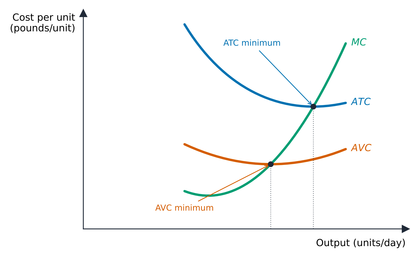
An additional unit costing less than the current average pulls the average down; one costing more pulls it up. In a smooth differentiable model, MC equals AVC at AVC's minimum and ATC at ATC's minimum. The two minima generally occur at different outputs.
Transfer question. A firm sells 10000 units/month at £10/unit. TFC is £40000/month and the firm makes only normal profit. Find AVC, including normal profit in economic costs.
Worked answer. Normal profit means zero economic profit, so TC equals TR:
$$TC=TR=P Q=\text{\pounds}10/\text{unit}\times10000\text{ units/month}=\text{\pounds}100000/\text{month}.$$
$$TVC=TC-TFC=\text{\pounds}100000/\text{month}-\text{\pounds}40000/\text{month}=\text{\pounds}60000/\text{month}.$$
$$AVC=\frac{TVC}{Q}=\frac{\text{\pounds}60000/\text{month}}{10000\text{ units/month}}=\text{\pounds}6/\text{unit}.$$
Here AR equals ATC, so subtracting AFC from price also gives AVC. That shortcut would fail if the firm earned supernormal or subnormal profit.
Long-run costs and scale

In the long run, no factor of production is fixed. Returns to scale 规模报酬 compare output when all inputs change in the same proportion, with technology unchanged. This differs from diminishing marginal returns, which changes the variable input while at least one other input remains fixed.
Worked example. A firm uses 100 workers and 2 machines to produce 1000 units/day. It doubles both inputs to 200 workers and 4 machines, producing 2500 units/day.
$$\text{Labour factor}=\frac{L_2}{L_1}=\frac{200\text{ workers}}{100\text{ workers}}=2.$$
$$\text{Capital factor}=\frac{K_2}{K_1}=\frac{4\text{ machines}}{2\text{ machines}}=2.$$
$$\text{Output factor}=\frac{Q_2}{Q_1}=\frac{2500\text{ units/day}}{1000\text{ units/day}}=2.5.$$
This is increasing returns to scale 规模报酬递增: output rises more than proportionately. With the same doubling of inputs, an output of 2000 units/day would show constant returns to scale 规模报酬不变; 1500 units/day would show decreasing returns to scale 规模报酬递减. These are alternative hypothetical results, not extra observations of this firm.
Physical returns and cost changes are linked only with suitable assumptions about input prices. Suppose the input bundle costs £10000/day initially and £20000/day after doubling, at unchanged input prices:
$$AC_1=\frac{TC_1}{Q_1}=\frac{\text{\pounds}10000/\text{day}}{1000\text{ units/day}}=\text{\pounds}10/\text{unit}.$$
$$AC_2=\frac{TC_2}{Q_2}=\frac{\text{\pounds}20000/\text{day}}{2500\text{ units/day}}=\text{\pounds}8/\text{unit}.$$
Economies of scale 规模经济 lower long-run average cost as scale increases. Here cost doubles while output rises by 2.5 times. If input prices change, the physical comparison alone does not determine the cost change. Compare the same product quality and technology; a cost reduction caused by new technology alone is not automatically caused by scale.
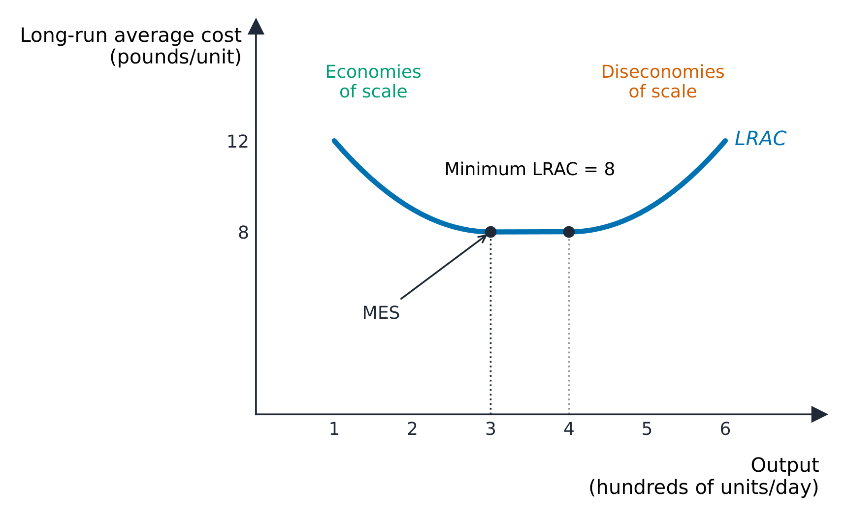
Long-run average cost (LRAC) is the lowest attainable average cost at each output when all inputs can be chosen. Minimum efficient scale 最小有效规模 (MES) is the smallest output at the minimum LRAC. It need not be the largest output shown, and a flat minimum can contain several equally efficient scales.
Worked example. Treat the following listed outputs as the available choices:
| Output (hundreds of units/day) | LRAC (£/unit) |
|---|---|
| 1 | 12 |
| 2 | 9 |
| 3 | 8 |
| 4 | 8 |
| 5 | 9 |
The minimum cost is £8/unit at both 300 and 400 units/day. MES is the first of these, 300 units/day. The following illustrative smooth model also has a flat minimum from 300 to 400 units/day. Diseconomies of scale 规模不经济 raise LRAC as scale increases beyond that range.
Internal and external scale effects
Classify the effect by whose expansion causes the cost change, then explain the mechanism:
- Internal economies of scale 内部规模经济 arise from the firm's own expansion. A specialised machine or division of tasks can increase output per resource. Bulk purchasing or cheaper finance can reduce input costs. The gain must lower cost per unit, not merely increase total output.
- External economies of scale 外部规模经济 arise from expansion of the industry. A larger local industry can support specialist suppliers, repair services or a pool of trained workers. A firm can gain even if its own size is unchanged.
- Internal diseconomies of scale 内部规模不经济 arise from the firm's expansion. More management layers, communication failures and weaker coordination can raise its unit cost.
- External diseconomies of scale 外部规模不经济 arise from industry expansion. Competition for local sites or skilled labour can bid up rents and wages; congestion can raise transport costs for several firms.
Internal/external here describes the source of a scale effect. It does not mean private/social cost, and a benefit to a neighbour is not automatically an external economy of scale: industry expansion must cause the cost reduction.
Spreading an unchanged fixed cost over more output is a short-run AFC effect, not by itself evidence of a long-run scale economy. AFC can fall while rising AVC causes ATC to rise. Long-run comparisons allow every input to change. Lower total cost alone proves neither lower average cost nor greater efficiency at a different quality of output.
Read average cost from long-run total cost
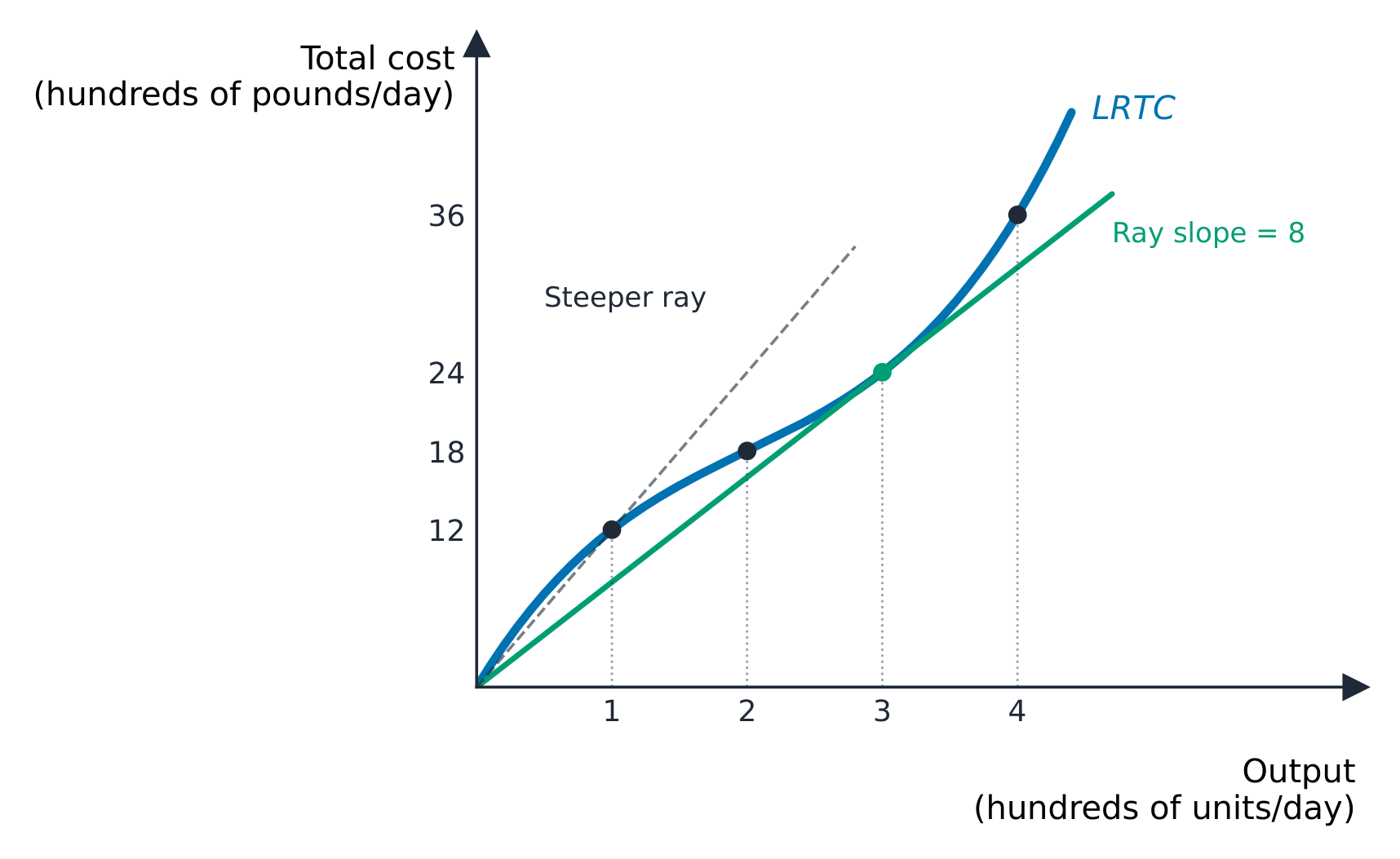
On a total-cost diagram, average cost is total cost divided by output: the slope of a straight ray from the origin to the point on the total-cost curve. The local slope of the curve instead measures marginal cost in a smooth model. Do not choose the flattest part of LRTC when asked for minimum LRAC.
Worked example. The following separate model has LRTC values of £1200, £1800, £2400 and £3600/day at 100, 200, 300 and 400 units/day. Divide each total by its own output to obtain LRAC values of £12, £9, £8 and £9/unit.
$$LRAC=\frac{LRTC}{Q}=\frac{\text{\pounds}2400/\text{day}}{300\text{ units/day}}=\text{\pounds}8/\text{unit}.$$
Revenue: separate totals, averages and changes
Total revenue 总收益 (TR) is all revenue from sales. Average revenue 平均收益 (AR) is revenue per unit sold. Marginal revenue 边际收益 (MR) is the additional revenue per extra unit of output. When the firm charges one price for all units:
$$TR=PQ,\qquad AR=\frac{TR}{Q}=P,\qquad MR=\frac{\Delta TR}{\Delta Q}.$$
Worked example. A firm sells 10 units/day at £50/unit. To sell 11 units/day it must lower the price to £48/unit on every unit.
$$TR_{10}=P_{10}Q_{10}=\text{\pounds}50/\text{unit}\times10\text{ units/day}=\text{\pounds}500/\text{day}.$$
$$TR_{11}=P_{11}Q_{11}=\text{\pounds}48/\text{unit}\times11\text{ units/day}=\text{\pounds}528/\text{day}.$$
$$AR_{11}=\frac{TR_{11}}{Q_{11}}=\frac{\text{\pounds}528/\text{day}}{11\text{ units/day}}=\text{\pounds}48/\text{unit}.$$
$$MR=\frac{\Delta TR}{\Delta Q}=\frac{(528-500)\text{\pounds/day}}{(11-10)\text{ units/day}}=\text{\pounds}28/\text{unit}.$$
The extra unit brings £48, but the price cut loses £2 on each of the previous ten units. Net revenue rises by only £28/day. MR is not the new selling price.
Contrast. A price taker can sell either 10 or 11 units/day at an unchanged £50/unit. With no price cut on earlier sales:
$$MR=\frac{\Delta TR}{\Delta Q}=\frac{(550-500)\text{\pounds/day}}{(11-10)\text{ units/day}}=\text{\pounds}50/\text{unit}.$$
An unchanged price gives MR=AR=P. With downward-sloping demand and a single price, MR is generally below AR because selling more requires a lower price on existing sales. With price discrimination, calculate actual total receipts; one common price cannot be assumed. Average revenue at zero sales is undefined.
Profit: include the opportunity cost of the owner's resources
Economic profit 经济利润 is total revenue minus all economic costs, including the opportunity cost of the owner's time and funds. Normal profit 正常利润 is the minimum required return that keeps the entrepreneur's resources in this use. It is counted within economic cost. Supernormal profit 超常利润 is profit above normal; subnormal profit 次正常利润 is a return below normal.
Worked example. Annual revenue is £24000 and explicit costs are £18000. The owner's time and funds have an implicit opportunity cost of £6000/year, with no other costs in this example:
$$TC=\text{explicit costs}+\text{opportunity costs}=\text{\pounds}18000/\text{year}+\text{\pounds}6000/\text{year}=\text{\pounds}24000/\text{year}.$$
$$\pi=TR-TC=\text{\pounds}24000/\text{year}-\text{\pounds}24000/\text{year}=0.$$
The firm makes normal profit: its required return is covered, so economic profit is zero. Accounting profit is £6000/year here because it omits that implicit cost. Zero economic profit does not mean the owner receives nothing.
For positive output, profit can also be calculated from the gap between average revenue and average total cost:
$$\pi=TR-TC=(AR-AC)Q.$$
Worked example. Keep output at 100 units/month and economic AC at £9/unit across three alternative revenue conditions:
$$\pi=(AR-AC)Q=(\text{\pounds}12/\text{unit}-\text{\pounds}9/\text{unit})\times100\text{ units/month}=\text{\pounds}300/\text{month}.$$
$$\pi=(AR-AC)Q=(\text{\pounds}9/\text{unit}-\text{\pounds}9/\text{unit})\times100\text{ units/month}=0.$$
$$\pi=(AR-AC)Q=(\text{\pounds}8/\text{unit}-\text{\pounds}9/\text{unit})\times100\text{ units/month}=-\text{\pounds}100/\text{month}.$$
These are supernormal, normal and subnormal profit respectively. Profit is the total gap over the period, not just the per-unit AR−AC difference.
Compare feasible output choices using profit
Try it. Only the following outputs are feasible in a separate daily example. Calculate profit for each row, then identify the best choice.
| Q (units/day) | TR (£/day) | TC (£/day) | Profit (£/day) |
|---|---|---|---|
| 0 | 0 | 4 | −4 |
| 1 | 10 | 8 | 2 |
| 2 | 18 | 13 | 5 |
| 3 | 24 | 19 | 5 |
| 4 | 28 | 26 | 2 |
Worked answer. Outputs 2 and 3 both maximise profit at £5/day. Increasing output from 2 to 3 gives:
$$\Delta\pi=\Delta TR-\Delta TC=(24-18)\text{\pounds/day}-(19-13)\text{\pounds/day}=0.$$
Across the successive one-unit steps, MR is £10, £8, £6 and £4/unit; MC is £4, £5, £6 and £7/unit. Profit rises when the extra revenue exceeds extra cost, is unchanged when they are equal, and falls when MC exceeds MR. The last unit raises total revenue but reduces profit. A discrete table can have a tie, so a unique output cannot always be inferred from MR=MC.
Profit levels and output decisions answer different questions
AR=AC means zero economic profit. It does not identify the output with the largest profit. MR=MC is a marginal condition: for a smooth interior maximum, marginal profit must change from positive to negative. Check feasible boundaries and stopping production too. With several intersections, compare total profit rather than assuming every MR=MC point is a maximum.

Worked example. In the graph, AR=14−Q, MR=14−2Q and MC=2+2Q, in £/unit, where Q is the numeric output in units/day. Total cost is £(10+2Q+Q²)/day. Marginal revenue exceeds marginal cost below 3 and falls below it above 3:
$$MR=MC\quad\Rightarrow\quad14-2Q=2+2Q\quad\Rightarrow\quad Q_\pi=3\text{ units/day}.$$
At 3 units/day, price is £11/unit, total revenue £33/day and total cost £25/day, giving profit £8/day. At either 1 or 5 units/day, revenue equals cost and profit is zero. This shows why a normal-profit question asks for the AR/AC intersection, not the MR/MC intersection.
A short-run loss and the decision to stop production
A negative economic profit does not automatically mean immediate closure is best. Some fixed costs may be unavoidable for the current period. Compare the loss from producing with the loss from stopping; keep long-run exit separate.
Worked example. Only 0 or 100 units/month are feasible this month. At 100 units, AVC is £4/unit and ATC is £6/unit. Fixed cost is £200/month and unavoidable; variable costs can be avoided by stopping. At a price of £5/unit:
$$\pi=(P-ATC)Q=(\text{\pounds}5/\text{unit}-\text{\pounds}6/\text{unit})\times100\text{ units/month}=-\text{\pounds}100/\text{month}.$$
Stopping gives no revenue and no variable cost, leaving the £200/month fixed-cost loss. Producing is preferable at this price because it covers variable cost and contributes to fixed cost. At a price of £3/unit:
$$\pi=(P-ATC)Q=(\text{\pounds}3/\text{unit}-\text{\pounds}6/\text{unit})\times100\text{ units/month}=-\text{\pounds}300/\text{month}.$$
Now stopping loses less. At a price equal to AVC, producing and stopping give the same loss under these assumptions. With more output choices, compare their contributions too. Long-run exit allows a new choice of all resources: reconsider avoidable costs, alternative opportunities and expected future returns rather than treating current fixed costs as unavoidable for ever.
Explore
Revenue & profit
y = ax² + bx + c
Total revenue rises then falls as price changes.
Explore
Costs and the firm
Average cost is U-shaped; marginal cost cuts it at the minimum. Different market structures price relative to these curves.
Explore
Average and marginal cost
Change output. Marginal cost cuts average cost at its lowest point — the heart of the theory of the firm.
Vocabulary
Train
| English |
|---|
| short run/ʃɔːt rʌn/ |
| long run/lɒŋ rʌn/ |
| fixed cost/fɪkst kɒst/ |
| variable cost/ˈveərɪəbl kɒst/ |
| total cost/ˈtəʊtl kɒst/ |
| diminishing returns/dɪˈmɪnɪʃɪŋ rɪˈtɜːnz/ |
| returns to scale/rɪˈtɜːnz tə skeɪl/ |
| economies of scale/ɪˈkɒnəmiz ɒv skeɪl/ |
| diseconomies of scale/ˌdɪsɪˈkɒnəmiz ɒv skeɪl/ |
| total revenue/ˈtəʊtl ˈrevənjuː/ |
| average revenue/ˈævrɪdʒ ˈrevənjuː/ |
| marginal revenue/ˈmɑːdʒɪnl ˈrevənjuː/ |
| normal profit/ˈnɔːml ˈprɒfɪt/ |
| supernormal profit/ˈsuːpənɔːml ˈprɒfɪt/ |
| subnormal profit/ˈsʌbnɔːml ˈprɒfɪt/ |
| total product/ˈtəʊtl ˈprɒdʌkt/ |
| average product/ˈævrɪdʒ ˈprɒdʌkt/ |
| marginal product/ˈmɑːdʒɪnl ˈprɒdʌkt/ |
| average fixed cost/ˈævrɪdʒ fɪkst kɒst/ |
| average variable cost/ˈævrɪdʒ ˈveərɪəbl kɒst/ |
| increasing returns to scale/ɪnˈkriːsɪŋ rɪˈtɜːnz tə skeɪl/ |
| constant returns to scale/ˈkɒnstənt rɪˈtɜːnz tə skeɪl/ |
| decreasing returns to scale/ˈdiːkriːsɪŋ rɪˈtɜːnz tə skeɪl/ |
| minimum efficient scale/ˈmɪnɪməm ɪˈfɪʃənt skeɪl/ |
| internal economies of scale/ɪnˈtɜːnl ɪˈkɒnəmiz ɒv skeɪl/ |
| external economies of scale/ekˈstɜːnl ɪˈkɒnəmiz ɒv skeɪl/ |
| internal diseconomies of scale/ɪnˈtɜːnl ˌdɪsɪˈkɒnəmiz ɒv skeɪl/ |
| external diseconomies of scale/ekˈstɜːnl ˌdɪsɪˈkɒnəmiz ɒv skeɪl/ |
| economic profit/ˌiːkəˈnɒmɪk ˈprɒfɪt/ |
7.6
Market structures
Syllabus
- explain the assumptions, behaviour and outcomes of perfect competition, monopolistic competition, oligopoly and monopoly
- explain price and non-price competition, collusion, price discrimination and the efficiency of each market structure
Source: Cambridge International syllabus
A market structure 市场结构 describes the number and size of sellers, entry conditions and the product sold. Define the product and geographical market before counting firms: a cafe may have no rival on one street but face rivals within walking distance.
| Structure | Sellers | Product | Entry conditions |
|---|---|---|---|
| perfect competition 完全竞争 | very many | identical | free entry and exit |
| monopolistic competition 垄断竞争 | many | differentiated | relatively easy |
| oligopoly 寡头垄断 | a few dominate | identical or different | substantial barriers |
| monopoly 垄断 | one | no close substitute | protected entry |
Product differentiation 产品差异化 means buyers see differences in quality, location, branding or service. It can give a firm some price-setting power. Barriers to entry 进入壁垒 include legal restrictions, difficult access to key inputs and cost advantages that a new supplier cannot readily match. They can help profit persist, but cannot guarantee profitable demand. A monopoly can make normal profit or a loss; an oligopoly need not form a cartel 卡特尔. Collusion 合谋 means firms coordinate decisions instead of acting independently. A cartel is an agreement between otherwise separate firms to restrict supply or fix prices. Potential competition must also be considered: a small number of current sellers does not by itself establish freedom from competitive pressure.
Worked classification. Many small farms selling the same grade of wheat at the market price fit perfect competition most closely. Many cafes with different menus and easy entry fit monopolistic competition. Three airlines that watch each other's fares and face expensive entry fit oligopoly. These are illustrative models, not claims that real markets meet every assumption. Reported profit alone does not identify structure.
Perfect competition: distinguish firm and market
A small price taker 价格接受者 accepts a market price that its own sales do not change. Market demand and supply determine this price. The individual firm's demand is horizontal at it; the whole market's demand curve is generally downward sloping.
At £10/unit, the firm sells 4 or 5 units/day:
$$TR_4=PQ=£10/\text{unit}\times4\text{ units/day}=£40/\text{day}$$
$$TR_5=PQ=£10/\text{unit}\times5\text{ units/day}=£50/\text{day}$$
$$AR_5=TR/Q=£50/\text{day}\div5\text{ units/day}=£10/\text{unit}$$
$$MR=\Delta TR/\Delta Q=(£50-£40)/1\text{ unit}=£10/\text{unit}$$
Thus $P=AR=MR$. Unlike the earlier price-cut example, an extra sale does not reduce the price received on previous sales. Find the best feasible output using marginal and total comparisons, not from the firm's name.
Short-run profit and shutdown
Worked comparison. In each separate case below, the best positive output is supplied as 4 units/day, TC is £40/day and TVC is £24/day. These are supplied case data, not a claim that a firm's optimum never changes when price changes. Use $TR=PQ$ and $\pi=TR-TC$.
| Price (£/unit) | TR (£/day) | TC (£/day) | Profit (£/day) |
|---|---|---|---|
| 12 | 48 | 40 | 8 |
| 10 | 40 | 40 | 0 |
| 8 | 32 | 40 | −8 |
All three outcomes are possible for a competitive firm in the short run. Zero economic profit includes the normal return on the owner's resources. Unavoidable fixed cost and average variable cost are:
$$TFC=TC-TVC=£40/\text{day}-£24/\text{day}=£16/\text{day}$$
$$AVC=TVC/Q=£24/\text{day}\div4\text{ units/day}=£6/\text{unit}$$
At £8/unit, production covers TVC and contributes £8/day towards fixed cost. The £8/day loss is smaller than the £16/day loss from stopping. In general compare the best positive-output contribution with stopping, allowing for which costs are actually avoidable. Do not use a short-run shutdown rule as an automatic long-run exit decision.
Entry, exit and the long-run competitive equilibrium
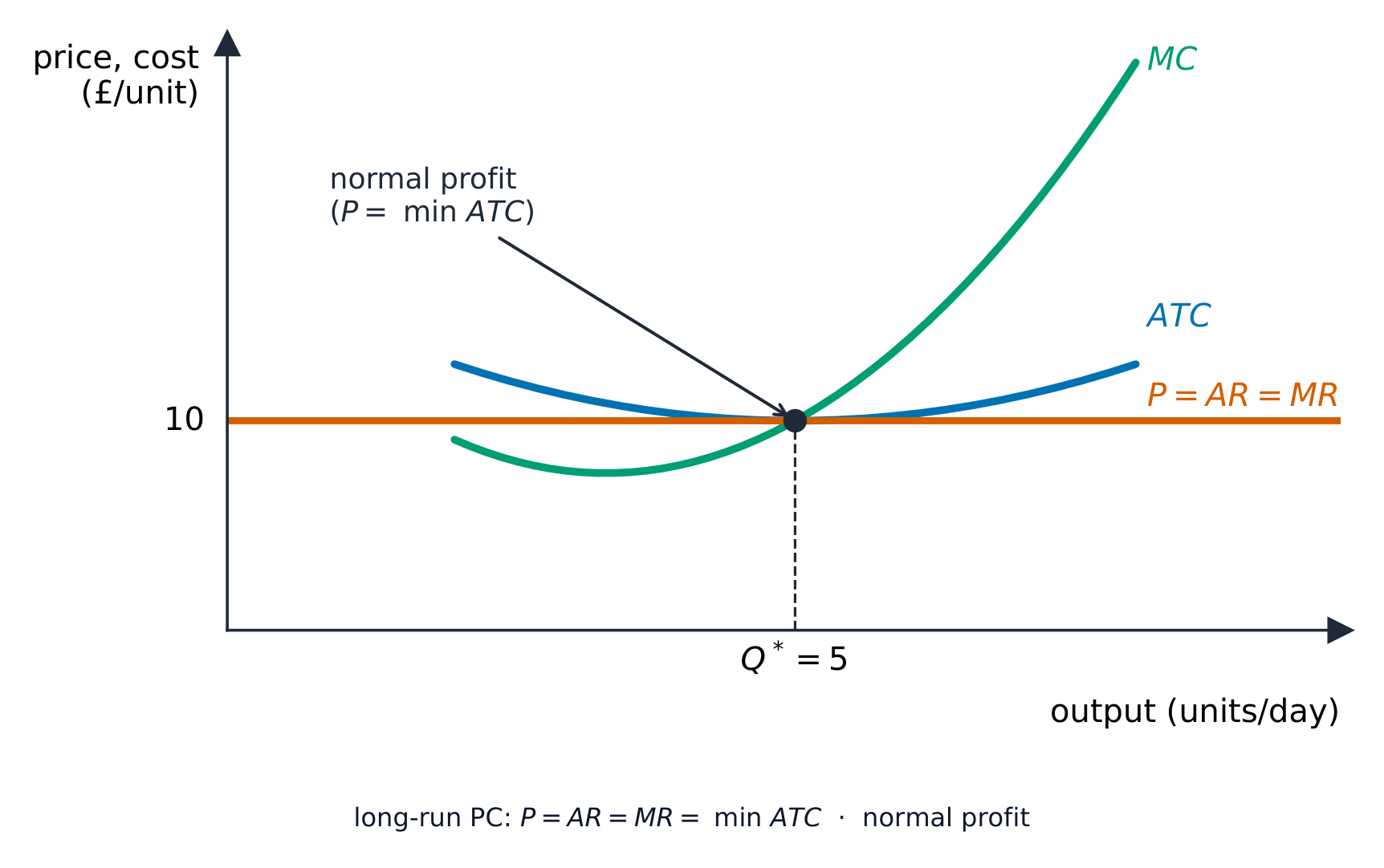
With free entry, economic profit attracts new firms. Market supply increases, tending to lower price and existing firms' profits. Losses encourage exit; reduced supply tends to raise price. This adjustment takes time. The familiar long-run result assumes unchanged conditions, informed buyers, access to the required inputs and technology, and no effective barriers to entry or exit. It is not a prediction that every observed farm earns exactly normal profit today.
The diagram uses $ATC=10+0.3(Q-5)^2$ and the consistent $MC=d(Q\times ATC)/dQ=17.5-6Q+0.9Q^2$. Costs are £/unit and output is units/day. At $Q=5$, ATC and rising MC are both £10/unit; the other lower-output MC intersection is not the maximum-profit choice. For this illustration the total-cost model is $TC=17.5Q-3Q^2+0.3Q^3$; it is separate from the earlier fixed-cost examples.
$$\pi=(P-ATC)Q=(£10-£10)/\text{unit}\times5\text{ units/day}=£0/\text{day}$$
Producing at minimum ATC is productive efficiency for the given technology and input prices. The equality $P=MC$ implies allocative efficiency only when price represents marginal benefit and private and social margins coincide. External effects or poor information can break this welfare conclusion. Neither normal profit nor a cost minimum alone proves dynamic efficiency: judge investment, finance and innovation incentives separately. Under the standard exam model, the absence of sustained supernormal profit can limit internal finance for research; this does not mean no competitive firm ever innovates.
Derive a firm's short-run supply
Worked discrete comparison. A different firm can produce only 0,1,2,3,4 units/day. TFC is £6/day, unavoidable in the short run; TVC is £0,£2,£6,£12,£20/day. Successive one-unit marginal costs are therefore £2,£4,£6,£8/unit. Compare all feasible outputs, including zero, at each price using $\pi=PQ-(TFC+TVC)$.
| Price (£/unit) | Best Q (units/day) | TR (£/day) | TC (£/day) | Profit (£/day) |
|---|---|---|---|---|
| 1 | 0 | 0 | 6 | −6 |
| 3 | 1 | 3 | 8 | −5 |
| 5 | 2 | 10 | 12 | −2 |
| 7 | 3 | 21 | 18 | 3 |
At £3, selling a second unit earns £3 but costs £4; adding it lowers profit. At £7, the fourth unit costs £8 and earns £7. Price below £2 leads to zero output; at £2 the firm is indifferent between zero and one unit. At prices £4,£6 and £8 the corresponding adjacent outputs tie. Do not force an equality rule on discrete steps when price lies between marginal costs.
For a conventional smooth cost model, the firm's short-run supply is the rising part of MC above minimum AVC. Below minimum AVC it supplies zero. At that minimum price it is indifferent between stopping and the best positive output. This assumes the indicated branch gives the best feasible contribution and fixed costs are unavoidable. Add the quantities supplied by firms at the same price to obtain industry supply. A monopoly's optimum depends on demand and MR as well as costs, so it has no equivalent price-only supply curve.
Monopoly: choose output, then read price and profit
A monopoly faces the market demand curve. An extra sale normally requires a lower price, so MR is below AR on the downward-sloping demand curve. Choosing a price does not let the firm sell any quantity it wants: its price and sales must be consistent with demand.
Worked model. Use $AR=P=18-Q$, $MR=18-2Q$ and $TC=20+2Q+Q^2$, with the consistent $MC=2+2Q$ and $ATC=20/Q+2+Q$. Output is units/day, price and marginal costs are £/unit and total cost is £/day. These numerical equations are an illustrative model, separate from the earlier competitive firm's cost curves.
At a smooth interior profit maximum:
$$MR=MC$$
$$18-2Q=2+2Q\quad\Rightarrow\quad Q=4\text{ units/day}$$
Read price from AR, not MR:
$$P=18-Q=18-4=£14/\text{unit}$$
$$TR=PQ=£14/\text{unit}\times4\text{ units/day}=£56/\text{day}$$
$$TC=20+2Q+Q^2=20+2(4)+4^2=£44/\text{day}$$
$$\pi=TR-TC=£56/\text{day}-£44/\text{day}=£12/\text{day}$$
The marginal difference $MR-MC=16-4Q$ is positive below 4 and negative above it. Thus the firm gains by expanding towards 4 from below and loses by expanding beyond 4. This quadratic profit model has a single positive-output maximum. Stopping loses the £20/day fixed cost if it is unavoidable; producing is better. For other cost/demand shapes, check all relevant branches, boundaries and feasible total profits.
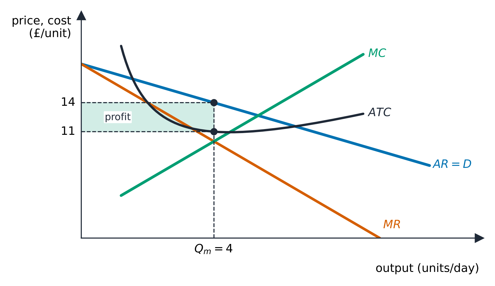
$$ATC=TC/Q=£44/\text{day}\div4\text{ units/day}=£11/\text{unit}$$
$$\pi=(P-ATC)Q=(£14-£11)/\text{unit}\times4\text{ units/day}=£12/\text{day}$$
The gap between price and MC is not profit per unit. It excludes some costs; use price minus ATC instead.
Entry barriers do not guarantee supernormal profit
Keep this demand and variable cost $TVC=2Q+Q^2$ unchanged but compare three alternative unavoidable fixed costs. The same MC implies the same optimum $Q=4$ and $P=£14$/unit in these particular cases.
| TFC (£/day) | TR (£/day) | TC (£/day) | Profit (£/day) |
|---|---|---|---|
| 20 | 56 | 44 | 12 |
| 32 | 56 | 56 | 0 |
| 40 | 56 | 64 | −8 |
At this output, variable cost is £24/day in every case. Changing unavoidable fixed cost shifts ATC and profit, but not MC here. The first monopoly earns supernormal profit, the second normal profit, and the third a loss. In the third case producing loses £8/day, whereas stopping loses £40/day, so production is preferable in the short run. If the cost becomes avoidable, or future demand changes, compare the long-run options again. Barriers can prevent entrants from competing a profit away; they cannot create sufficient demand or remove a firm's costs.
Compare profit maximisation with the social margin
With no external effects or information problems, suppose the demand price represents marginal social benefit and MC represents marginal social cost. At the monopoly output of 4, buyers value a small extra unit at £14 while it costs £10 to supply. Extra output can therefore add net social benefit even though it reduces the monopoly's profit.
The illustrative social optimum uses $MSB=MSC$, not $MR=MC$:
$$MSB=MSC$$
$$18-Q=2+2Q\quad\Rightarrow\quad Q^*=16/3\text{ units/day}\approx5.33\text{ units/day}$$
$$P^*=18-Q^*=18-16/3=£38/3\text{ per unit}\approx£12.67/\text{unit}$$
This compares outcomes using unchanged demand and costs, without other distortions. It is not a claim that every price control will work: a real policy must consider information, cost recovery, investment incentives and implementation. Nor does monopoly status prove poor innovation or inefficient management; investigate costs, incentives and evidence.
Monopolistic competition: entry, normal profit and excess capacity
Many sellers offer differentiated products, with relatively easy entry and exit. Buyers may not know every quality difference or price. Each firm faces a downward-sloping demand curve because it can lose customers to close substitutes; some price-setting power does not mean unlimited freedom to raise price. In the short run, demand and costs can give profit or loss. In the standard long-run model, profit attracts entry of close substitutes, reducing each incumbent's demand until economic profit is zero. Losses encourage exit. The remaining firm's demand does not become horizontal merely because entry is free.
Worked long-run illustration. Keep $AR=18-Q$, $MR=18-2Q$ and $MC=2+2Q$, but use $TC=32+2Q+Q^2$. At $Q=4$ units/day, $MR=MC$ and price read from AR is £14/unit:
$$TC=32+2Q+Q^2=32+2(4)+4^2=£56/\text{day}$$
$$ATC=TC/Q=£56/\text{day}\div4\text{ units/day}=£14/\text{unit}$$
$$\pi=(P-ATC)Q=(£14-£14)/\text{unit}\times4\text{ units/day}=£0/\text{day}$$
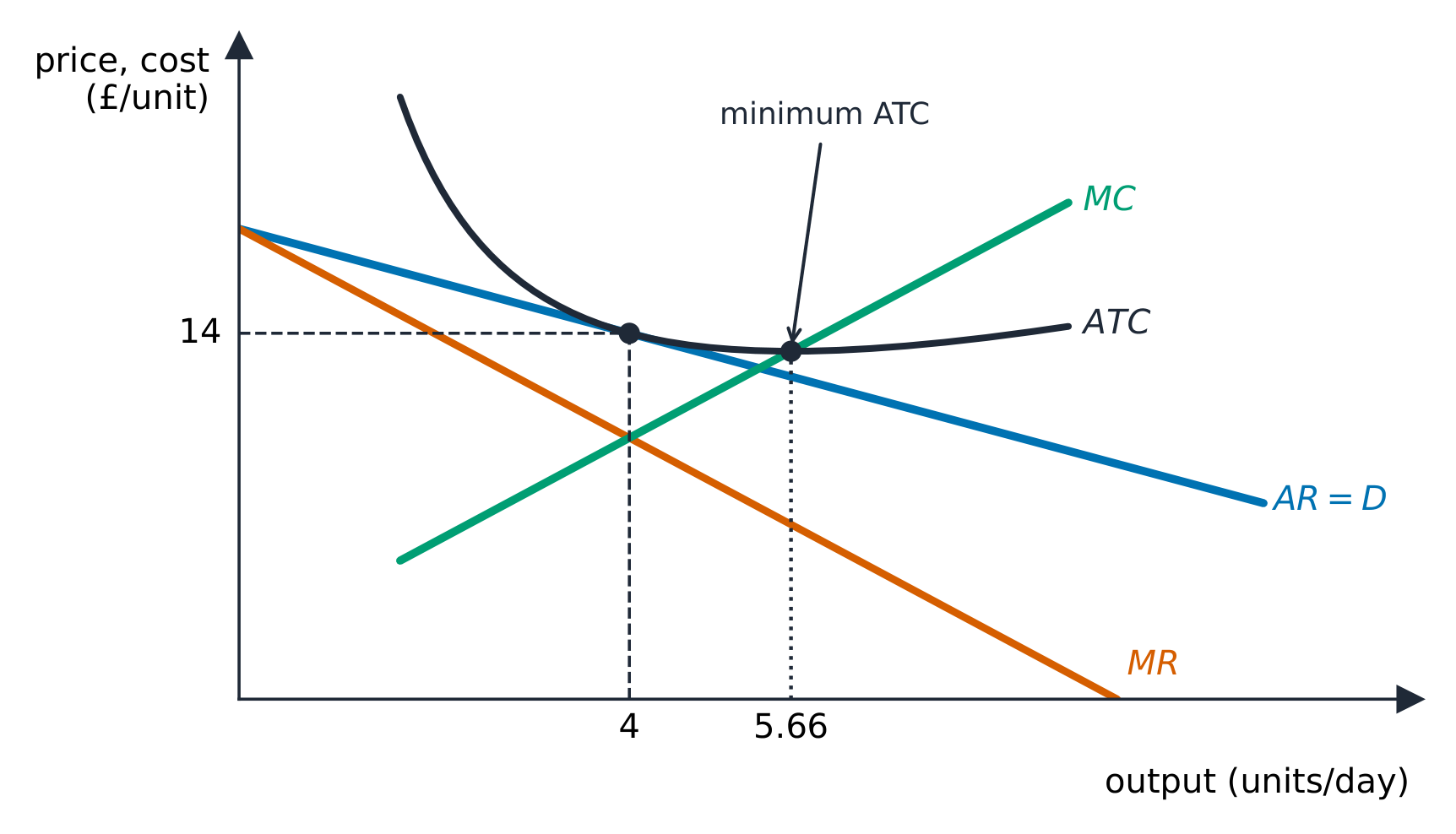
Here $ATC=32/Q+2+Q$. At output 5 it is £13.40/unit, already below £14/unit at 4; the minimum is about £13.31/unit at output 5.66. Thus the firm has excess capacity relative to the output minimising ATC in this model. Also $P=14>MC=10$, so the private marginal condition for allocative efficiency is not met. Free entry and normal profit do not make this the same outcome as perfect competition. Product variety may benefit buyers; weigh that benefit rather than assuming that identical products must always be best.
Natural monopoly and the relevant cost range
A natural monopoly 自然垄断 exists when one firm can supply the relevant market at lower total cost than multiple firms. A large network cost and falling LRAC over the range of market demand can produce this condition. It is a cost argument, not simply a statement that one seller happens to exist.
Worked network. Market demand is 100 identical service units/month. Each active network requires £120/month of overhead plus £2/unit supplied. Treat these as the least feasible costs of a network in this illustration, allowing a provider to close; two providers require two separate networks. Quality and input prices are identical.
$$TC_{\text{one}}=120+2Q=120+2(100)=£320/\text{month}$$
$$TC_{\text{two}}=2[120+2(50)]=£440/\text{month}$$
$$AC_{\text{one}}=TC_{\text{one}}/Q=£320/\text{month}\div100\text{ units/month}=£3.20/\text{unit}$$
$$AC_{\text{two}}=TC_{\text{two}}/Q=£440/\text{month}\div100\text{ units/month}=£4.40/\text{unit}$$
Duplicating the network adds £120/month. Over this relevant demand range, one provider has the lower total cost. This does not justify any price it chooses or prove good management. A larger market, different technology or shared network access may change the comparison. Regulation must consider service standards, cost recovery and investment as well as price.
X-inefficiency: avoidable cost at a given output
X-inefficiency X低效率 means avoidable costs above a feasible best-practice cost for the same output. Weak pressure to control costs may permit waste, poor supervision or slack management, but neither monopoly status nor a high observed cost proves this on its own.
Worked comparison. A network supplies 100 service units/month at an actual cost of £440/month. A feasible best-practice method costs £320/month, with the same input prices, quality and reliability:
$$\text{Avoidable cost}=TC_{\text{actual}}-TC_{\text{best}}=£440/\text{month}-£320/\text{month}=£120/\text{month}$$
$$\text{Gap per unit}=\text{Avoidable cost}/Q$$
$$\text{Gap per unit}=£120/\text{month}\div100\text{ units/month}=£1.20/\text{unit}$$
A costly remote location or higher quality might instead explain higher costs without avoidable inefficiency. Control those differences before drawing the conclusion. Producing away from minimum ATC concerns output choice along a cost curve. X-inefficiency concerns avoidable cost above the feasible curve at a given output. These are different tests.
Concentration ratios: combined shares of the largest firms
A concentration ratio 集中度 is the combined market share of a specified number of the largest firms. Define the product, geographical market, period and measure, such as sales revenue. Use a consistent measure in both numerator and denominator.
Worked four-firm ratio. Firms A–F have annual sales of £60m, £50m, £40m, £20m, £16m and £14m. Total market sales are £200m/year. The largest four have £170m/year:
$$CR_4=\frac{\text{sales of largest four}}{\text{total market sales}}\times100$$
$$CR_4=\frac{(60+50+40+20)\text{ £m/year}}{200\text{ £m/year}}\times100=85\%$$
Now A and B merge and all sales stay unchanged. The merged firm has £110m/year, followed by firms with £40m, £20m, £16m and £14m. Re-rank before selecting the largest four:
$$CR_{4,\text{after}}=\frac{(110+40+20+16)\text{ £m/year}}{200\text{ £m/year}}\times100=93\%$$
All numerator and denominator values use £million/year. The increase is 8 percentage points. Do not count A and B separately after they merge; do not confuse an 85% combined share with 85% for each firm. High concentration shows dominance by a few large sellers but does not alone prove collusion, high prices or weak potential entry.
Entry, exit and contestability
Explain how a barrier works. A restrictive licence is a legal barrier. A scarce suitable harbour site is a physical obstacle. An incumbent's large low-cost network may give a cost advantage that a smaller entrant cannot match. Strong buyer loyalty to an established brand is a market obstacle. Categories can overlap; the mechanism matters more than assigning a single label. Perfect competition assumes many buyers and sellers, informed choices, an identical product and free entry and exit. Few sellers with imperfect information may have a different competitive position even when other features look similar.
A contestable market 可竞争市场 faces effective pressure from potential entrants. In the ideal model, entry and exit are free, entrants can access comparable technology and costs, and there are no unrecoverable entry costs. Even a few current sellers may keep prices close to cost if a newcomer can quickly win business and leave without a large loss. The number of current firms is therefore not a complete test of competition. A temporary profit opportunity is less threatening if entering takes years or incumbents can react before entrants recover their investment.
A sunk cost 沉没成本 is unrecoverable once incurred. It is different from a fixed cost, which describes how cost varies with output during a period. Equipment that can be sold on exit is not wholly sunk.
Worked entry investment. A newcomer spends £20,000 on equipment and £5,000 on launch advertising. It can resell the equipment for £18,000 on exit; the advertising cannot be recovered. Ignoring other costs and receipts:
$$\text{Sunk cost}=\text{initial outlay}-\text{recoverable value}$$
$$\text{Sunk cost}=(£20{,}000+£5{,}000)-£18{,}000=£7{,}000$$
This £7,000 makes quick entry and exit less attractive than the full-recovery case. Once already incurred, however, sunk cost should not itself justify continued production: compare future avoidable costs and returns. Future exit penalties and obligations may affect that comparison. Do not claim that past sunk spending automatically traps a firm into rationally operating at a continuing avoidable loss.
Oligopoly: interdependent choices and a payoff matrix
In oligopoly, a few firms dominate and each firm's outcome depends on how rivals respond. Firms may compete on price, service or quality, or coordinate decisions. Neither collusion nor a price war is inevitable. A payoff matrix 收益矩阵 lists each player's outcome for every combination of choices.
Illustrative one-shot game. Two firms independently and simultaneously choose high or low prices, without a binding agreement. Each cell gives (A's profit, B's profit) in £/week. These are teaching data, not a prediction of actual airline or cafe profits.
| A's choice | B: high | B: low |
|---|---|---|
| High | (700, 700) | (200, 900) |
| Low | (900, 200) | (400, 400) |
Read the first number for A and the second for B. If B chooses high, A prefers low: £900/week rather than £700/week. If B chooses low, A still prefers low: £400/week rather than £200/week. The symmetric reasoning gives the same preferred responses for B. Thus both choose low, making £400/week each. Neither can improve by changing alone from low/low.
Yet high/high would give £700/week each. This is a Prisoner's Dilemma 囚徒困境: each firm's individually preferred response produces an outcome worse for both than mutual cooperation in this table.
$$\text{Joint profit}_{HH}=£700/\text{week}+£700/\text{week}=£1{,}400/\text{week}$$
$$\text{Joint profit}_{LL}=£400/\text{week}+£400/\text{week}=£800/\text{week}$$
The higher joint total does not remove the temptation for one firm to undercut while the other keeps a high price. A cartel must address incentives, monitoring and responses to cheating. New entrants, differing costs and many participants can weaken coordination. Repeated dealings and credible future responses may change incentives; the one-shot result is conditional on the displayed payoffs and assumptions. Do not infer one universal outcome for every oligopoly.
Price and non-price competition: compare profits, not only sales
Price competition 价格竞争 means changing price to attract buyers. Non-price competition 非价格竞争 uses quality, service, branding or promotion. Advertising can communicate useful differences or build loyalty; better service may increase costs as well as demand. Rivals may imitate either approach, so neither is guaranteed to succeed.
Worked monthly forecasts. Initially price is £10/unit, sales are 100 units/month, unit variable cost is £6 and fixed cost is £200/month. A price cut to £9 is forecast to sell 115 units/month with the same fixed cost. Alternatively, price stays £10 and extra service/advertising costing £60/month is forecast to raise sales to 120 units/month. Use $TR=PQ$, $TC=TFC+vQ$ and $\pi=TR-TC$, where $v=£6$/unit.
| Case | Q | TR | TC | Profit |
|---|---|---|---|---|
| Initial | 100 | 1000 | 800 | 200 |
| Price cut | 115 | 1035 | 890 | 145 |
| Service/ad | 120 | 1200 | 980 | 220 |
Output is units/month; money totals are £/month. The price cut increases revenue by £35/month but reduces profit by £55/month. The service/advertising forecast increases profit by £20/month after its extra cost. For example:
$$TC_{\text{ad}}=TFC+vQ=£260/\text{month}+£6/\text{unit}\times120\text{ units/month}=£980/\text{month}$$
$$\pi_{\text{ad}}=TR-TC=£1{,}200/\text{month}-£980/\text{month}=£220/\text{month}$$
These are forecasts. If rivals match the offer or demand disappoints, recalculate rather than assuming the stated sales increase. A price reduction may benefit buyers even if it reduces the firm's profit.
Price discrimination: distinguish the pricing rule
Price discrimination 价格歧视 means different prices for the same product where the difference is not explained by different supply costs. A higher delivery charge for a distant address may reflect a higher cost, so different prices alone do not prove discrimination. A ticket bought early and a ticket bought just before departure may sort travellers by their willingness to pay; changing demand or capacity also needs consideration. Do not infer the precise degree from timing alone.
- First-degree price discrimination 一级价格歧视 charges each unit at the individual buyer's maximum willingness to pay for that unit. It requires detailed information and control over resale; it is an idealised benchmark, not simply charging one high price to everyone.
- Second-degree price discrimination 二级价格歧视 varies the unit price with quantity or a menu of purchase options. Buyers select an option rather than the seller assigning a price from their identity. A quantity discount is discriminatory only insofar as its price differences are not explained by cost differences.
- Third-degree price discrimination 三级价格歧视 charges different identifiable groups different prices for the same product, for example an ID-checked student ticket and an adult ticket. Groups must be kept separate. Different demand responses allow different profit-maximising mark-ups; it is not necessary for every group to have inelastic demand.
Compare a uniform price with first-degree pricing
Illustrative three-unit model. One buyer is willing to pay up to £12 for the first unit, £9 for the second and £6 for the third. Additional units have no value to this buyer. Each unit costs £4 to supply, there is no fixed cost, and the buyer purchases when willingness to pay is at least the price. Ignore administration costs initially.
| Uniform price (£/unit) | Units bought | TR (£) | Cost (£) | Profit (£) |
|---|---|---|---|---|
| 12 | 1 | 12 | 4 | 8 |
| 9 | 2 | 18 | 8 | 10 |
| 6 | 3 | 18 | 12 | 6 |
These willingness-to-pay thresholds give the best uniform prices for each possible positive quantity. A higher price within a range cannot sell more; lowering it within that range only reduces revenue. Not selling gives zero profit. The best uniform choice is therefore £9/unit and two units, with profit £10.
Under first-degree pricing the seller charges £12, £9 and £6 for the three units. All three units' marginal values here exceed the £4 marginal cost:
$$TR=\sum P_i=£12+£9+£6=£27.$$
$$TC=MC\times Q=(£4/\text{unit})(3\text{ units})=£12.$$
$$\pi=TR-TC=£27-£12=£15.$$
The uniform-price buyer keeps £3 of consumer surplus on the first unit. Perfect first-degree pricing takes that surplus and also serves the third unit. Consumer surplus is zero under the stated purchase-at-indifference assumption. With marginal willingness to pay representing social benefit, marginal cost representing social cost and no other distortion, supplying the third unit adds £2 of total surplus. This efficiency result does not establish a fair distribution or that perfect information is realistic.
Second-degree pricing: let the buyer choose a quantity
Keep the same buyer and constant £4/unit cost. Offer the first two units at £9 each and the third at £5. The total bill is £9 for one, £18 for two and £23 for three. The buyer's total willingness to pay is £12, £21 and £27 respectively. Net benefits are £3, £3 and £4, so the buyer strictly prefers three units. This is a quantity menu, not a price based on a student ID.
$$\pi=TR-TC=£23-(£4/\text{unit})(3\text{ units})=£11.$$
Profit is £1 above the best uniform-price profit. Extra administration cost above £1 removes that gain. The constant cost assumption makes clear that this price pattern is not simply passing on a cheaper cost of supplying the third unit. A different buyer may choose another quantity; the menu does not force everyone to buy three.
Third-degree pricing: separate identifiable groups
A separate illustrative market. Each customer buys at most one visit; cost is £4/visit, with no fixed or administration cost. In group A two customers will pay up to £12 and £10. In group B two will pay up to £7 and £5. Customers buy at a price equal to their maximum willingness to pay. Group membership can be verified and tickets cannot be transferred.
| One price (£/visit) | Visits sold | TR (£) | Profit (£) |
|---|---|---|---|
| 12 | 1 | 12 | 8 |
| 10 | 2 | 20 | 12 |
| 7 | 3 | 21 | 9 |
| 5 | 4 | 20 | 4 |
The best uniform price is £10, giving two visits and £12 profit. For separate group prices, A's best choice is £10 for two visits, giving £12 profit. B's best choice is £7 for one visit, giving £3 profit, rather than £5 for two visits giving £2 profit. Together:
$$TR=P_AQ_A+P_BQ_B=(£10/\text{visit})(2\text{ visits})+(£7/\text{visit})(1\text{ visit})=£27.$$
$$TC=MC(Q_A+Q_B)=(£4/\text{visit})(3\text{ visits})=£12.$$
$$\pi=TR-TC=£27-£12=£15.$$
One extra B customer is served and profit rises by £3 before administration costs. This numerical result does not imply that all customers gain or that discrimination always expands output. The values are illustrative thresholds, not estimates of demand elasticities. In the usual smooth third-degree model with a common marginal cost, the group with less elastic demand at its chosen price bears a higher mark-up. Apply that rule to the relevant demand response rather than assuming age or income alone proves elasticity.
Conditions and consequences: test the mechanism
Effective discrimination requires some price-setting power, information that allows useful prices or options to be set, and limits on resale or switching between prices. Third-degree group pricing additionally needs identifiable, separable segments with different demand responses. A full single-seller monopoly is not required; price leadership is not a necessary condition. ID checks, non-transferable services or quantity menus may help, but verification costs and customer behaviour matter.
If any adult can buy a transferable student ticket and resell it, the higher-price group can bypass the adult price. Cheap resale undermines separation. An ID check may reduce that route, but its cost and enforcement determine whether it works. A firm that guesses willingness to pay badly can lose buyers; the original uniform price remains an available alternative only if the firm can choose it and avoid extra costs.
Compare the whole outcome with a feasible alternative. Some buyers may pay more, others may gain access at a lower price. Output can rise, fall or remain unchanged, so the effect on allocative efficiency is conditional. Perfect first-degree pricing can remove the restricted-output loss under the benchmark assumptions above while transferring consumer surplus to the firm. Third-degree pricing does not in general remove that loss. Higher profit might finance investment or keep a service operating, but neither follows automatically. Administration costs, information limits, resale and entry can reduce or remove the gain. Judge profit, access, efficiency and distribution separately.
Explore
Pricing and competition
How a firm prices depends on demand and supply; with market power it can charge above the competitive level.
Vocabulary
Train
| English |
|---|
| market structure/ˈmɑːkɪt ˈstrʌktʃə/ |
| perfect competition/ˈpɜːfekt ˌkɒmpəˈtɪʃn/ |
| monopolistic competition/məˈnɒpəlɪstɪk ˌkɒmpəˈtɪʃn/ |
| oligopoly/ˌɒlɪˈɡɒpəli/ |
| monopoly/məˈnɒpəli/ |
| price taker/praɪs ˈteɪkə/ |
| product differentiation/ˈprɒdʌkt ˌdɪfəˌrenʃɪˈeɪʃn/ |
| collusion/kəˈluːʒn/ |
| cartel/kɑːˈtel/ |
| barriers to entry/ˈbærɪəz tʊ ˈentri/ |
| price competition/praɪs ˌkɒmpəˈtɪʃn/ |
| non-price competition/nɒn praɪs ˌkɒmpəˈtɪʃn/ |
| price discrimination/praɪs dɪˌskrɪmɪˈneɪʃn/ |
| natural monopoly/ˈnætʃərəl məˈnɒpəli/ |
| X-inefficiency/eks ɪnɪˈfɪʃənsi/ |
| concentration ratio/ˌkɒnsənˈtreɪʃn ˈreɪʃɪəʊ/ |
| contestable market/kənˈtestəbl ˈmɑːkɪt/ |
| sunk cost/sʌŋk kɒst/ |
| payoff matrix/ˈpeɪɒf ˈmeɪtrɪks/ |
| Prisoner's Dilemma/ˈprɪzənəz daɪˈlemə/ |
| first-degree price discrimination/fɜːst dɪˈɡriː praɪs dɪˌskrɪmɪˈneɪʃn/ |
| second-degree price discrimination/ˈsekənd dɪˈɡriː praɪs dɪˌskrɪmɪˈneɪʃn/ |
| third-degree price discrimination/θɜːd dɪˈɡriː praɪs dɪˌskrɪmɪˈneɪʃn/ |
7.7
The growth and survival of firms
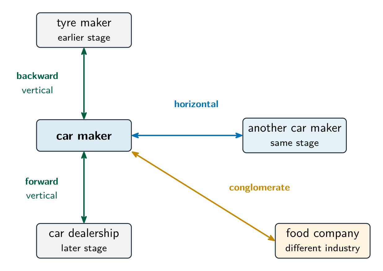
Syllabus
- explain why firms grow (internal and external — horizontal, vertical, conglomerate integration) and why some remain small
- explain barriers to entry and exit and the survival of small firms
Source: Cambridge International syllabus
A firm may expand to meet growing demand, reduce unit cost, gain bargaining power, secure supplies or enter a new market. Its size also depends on finance, management capacity, technology, the size of its market and the owner's objectives. None of these makes growth automatically profitable or socially beneficial.
Internal growth, external growth and diversification
Internal growth 内部增长, also called organic growth 有机增长, expands a business through its own investment and activities: employing staff, adding equipment, opening branches or developing products. A bakery opening its own second shop is an example. Higher sales may follow, but simply defining growth as selling more omits the investment and capacity decisions.
Diversification 多元化经营 expands into a different product or market. It can be internal: a car maker develops its own food business without buying another firm. It can also be external, through acquiring a business in another industry. Diversification and the method of growth answer different questions.
External growth 外部增长 combines existing businesses through a merger 合并 or takeover 收购. A takeover transfers control of another business; it is different from building an additional branch. Combining two existing businesses can increase capacity quickly, but integration takes time and resources. Growing internally can allow closer control over development, but may be slower or limited by available finance and skills. Judge the actual plans rather than assuming one method is always better.
Integration: start from the acquiring firm's position
Worked classification. A car maker buys four different businesses in four separate cases:
- Another car maker: horizontal integration 横向一体化, combining firms at the same stage of the same industry.
- A tyre supplier: backward vertical integration 后向纵向一体化, moving towards an earlier input-supply stage.
- A car dealership: forward vertical integration 前向纵向一体化, moving towards distribution and final buyers.
- A food company: conglomerate integration 混合一体化, combining businesses in different industries. This is external diversification.
Backward and forward are both vertical integration 纵向一体化: different stages of the same production chain are combined. Reversing who buys whom reverses the direction. A tyre supplier buying a car maker moves forward; a dealership buying a car maker moves backward. Draw the chain and identify the buyer before naming the type.
A horizontal merger may share specialist equipment, remove duplicated costs and increase bargaining power, but also reduce competitive pressure. Backward integration may secure supplies and quality; forward integration may secure distribution and information about buyers. Both can introduce unfamiliar management tasks or reduce flexibility in choosing other suppliers. Conglomerate integration may spread exposure across markets, but risks can remain linked and management may lack experience in the new industry. Explain a specific mechanism and its limits instead of saying that every merger achieves economies of scale.
Compare merger savings with costs and stakeholder effects
Worked monthly forecast. Two firms together sell 200 units/month at £6/unit. Their combined cost is £1,000/month. A merger is forecast to reduce recurring cost to £800/month at the same output and quality, but there is a £300 transition bill in its first month. Use $AC=TC/Q$, $TR=PQ$ and $\pi=TR-TC$.
$$TR=PQ=£6/\text{unit}\times200\text{ units/month}=£1{,}200/\text{month}$$
| Case | TC (£/month) | AC (£/unit) | Profit (£/month) |
|---|---|---|---|
| Before | 1000 | 5.00 | 200 |
| First month | 1100 | 5.50 | 100 |
| Later month | 800 | 4.00 | 400 |
The first-month cost includes the transition payment:
$$TC_{\text{first}}=TC_{\text{recurring}}+\text{transition cost}=£800/\text{month}+£300/\text{month}=£1{,}100/\text{month}$$
$$AC_{\text{first}}=TC_{\text{first}}/Q=£1{,}100/\text{month}\div200\text{ units/month}=£5.50/\text{unit}$$
$$\pi_{\text{first}}=TR-TC_{\text{first}}=£1{,}200/\text{month}-£1{,}100/\text{month}=£100/\text{month}$$
Later recurring savings are conditional on the forecast being achieved. Lost customers, incompatible systems or management problems can change them. This operating-cost illustration is not a full investment appraisal: acquisition price, financing and opportunity costs also matter. Compare the same period, output and quality rather than hiding a one-off bill in a different period.
Lower costs need not mean lower prices if market power increases. Buyers may gain from quality or lower prices, or lose from reduced choice and higher prices. Workers may face training opportunities or job losses; suppliers may gain stable contracts or face stronger bargaining pressure. Owners' profit is only one part of the assessment.
Why small firms survive and why some choose not to grow
A specialist repairer may have limited local demand and provide personal service with few scale economies. That does not mean every local service has no route to expansion: another profitable location, a new service model or a franchise may permit growth. An online craft seller can reach a large geographical market and still choose to stay small to keep control. A supplier can remain small by meeting specialised orders from large manufacturers reliably.
A niche 利基市场 is a narrow customer need or market segment. Distinctive products, personal service, flexibility and supplying larger firms can help a small firm survive. They do not guarantee profit: easy entry may attract rivals, and customers' needs can change. Finance, management capacity, demand and the cost path constrain the decision to expand. Small size is not by itself evidence of failure; large size is not proof of efficiency.
Barriers to exit 退出壁垒 include future penalties or obligations that make leaving costly. Past sunk spending is different. Once a machine's unrecoverable purchase cost is already sunk, that spending alone should not justify continued avoidable losses. Compare future avoidable costs, receipts, exit obligations and alternative opportunities.
Effective cartels: conditions and consequences
Revisit the earlier payoff matrix. A high joint profit does not remove each firm's incentive to undercut or supply more than its agreed quantity. A small number of firms can make coordination easier, similar costs can make preferred prices more alike, and observable sales can make cheating easier to detect. Stable demand can help distinguish cheating from an unexpected change in orders. Barriers to entry reduce the threat of outside suppliers taking profitable business.
Worked comparison. Industry A has three similar-cost firms, stable demand, observable sales and difficult entry. Industry B has twenty different-cost firms, volatile orders, hard-to-observe sales and easy entry. A has more favourable conditions for maintaining a supply agreement, but it is not guaranteed to do so. B faces more coordination problems, conflicting preferred prices, difficult monitoring and outside entry. High concentration by itself does not establish a stable cartel.
An effective supply restriction can raise prices and member profits while reducing output and buyer choice. Where no other distortion offsets the restriction, output below the social optimum can cause a welfare loss. Cheating, entry or changed costs and demand can undermine the agreement. Evaluate the mechanism and the evidence, not the label alone.
Owners, managers and the principal-agent problem
The principal-agent problem 委托代理问题 arises when a person making decisions has different incentives from the person represented, especially when actions or effort are hard to observe. The divorce of ownership from control 所有权与控制权分离 can create this problem: shareholders own a large company while managers make many decisions. Conflict is possible, not inevitable; owners' objectives can differ too.
Worked incentives. Project A produces £10,000/month profit before bonuses and offers the manager an easier schedule. B produces £12,000/month before bonuses but needs more supervision. The manager receives the same fixed salary in either case. A profit-seeking owner prefers B here; the manager may prefer A's easier schedule. A 10% profit bonus gives:
$$\text{Bonus}_A=0.10\times\text{profit}_A=0.10\times£10{,}000/\text{month}=£1{,}000/\text{month}$$
$$\text{Bonus}_B=0.10\times\text{profit}_B=0.10\times£12{,}000/\text{month}=£1{,}200/\text{month}$$
B gives the manager £200/month more bonus. Owners also prefer B after these bonuses: retained profit is £10,800/month rather than £9,000/month, before any unchanged salary already accounted for in the original profit figures. The incentive narrows the conflict but does not guarantee alignment: an easier schedule could be worth more than £200/month to the manager.
Monitoring, profit-related pay and longer-term share incentives can help. They also have costs and can encourage manipulation of short-term targets or risky choices. Choose a measure that reflects the intended outcome and check behaviour rather than assuming any bonus solves the problem completely.
Explore
Firm objective lab
Classify real firm decisions by the objective they reveal.
Vocabulary
Train
| English |
|---|
| internal growth/ɪnˈtɜːnl ɡrəʊθ/ |
| external growth/ekˈstɜːnl ɡrəʊθ/ |
| merger/ˈmɜːdʒə/ |
| horizontal integration/ˌhɒrɪˈzɒntl ˌɪntɪˈɡreɪʃn/ |
| vertical integration/ˈvɜːtɪkl ˌɪntɪˈɡreɪʃn/ |
| conglomerate integration/kənˈɡlɒməreɪt ˌɪntɪˈɡreɪʃn/ |
| niche/niːʃ/ |
| barriers to exit/ˈbærɪəz tʊ ˈeɡzɪt/ |
| divorce of ownership from control/dɪˈvɔːs ɒv ˈəʊnəʃɪp frɒm kənˈtrəʊl/ |
| principal-agent problem/ˈprɪnsɪpl ˈeɪdʒənt ˈprɒbləm/ |
| organic growth/ɔːˈɡænɪk ɡrəʊθ/ |
| diversification/daɪˌvɜːsɪfɪˈkeɪʃn/ |
| takeover/ˈteɪkəʊvə/ |
| backward vertical integration/ˈbækwəd ˈvɜːtɪkl ˌɪntɪˈɡreɪʃn/ |
| forward vertical integration/ˈfɔːwəd ˈvɜːtɪkl ˌɪntɪˈɡreɪʃn/ |
7.8
The objectives of firms
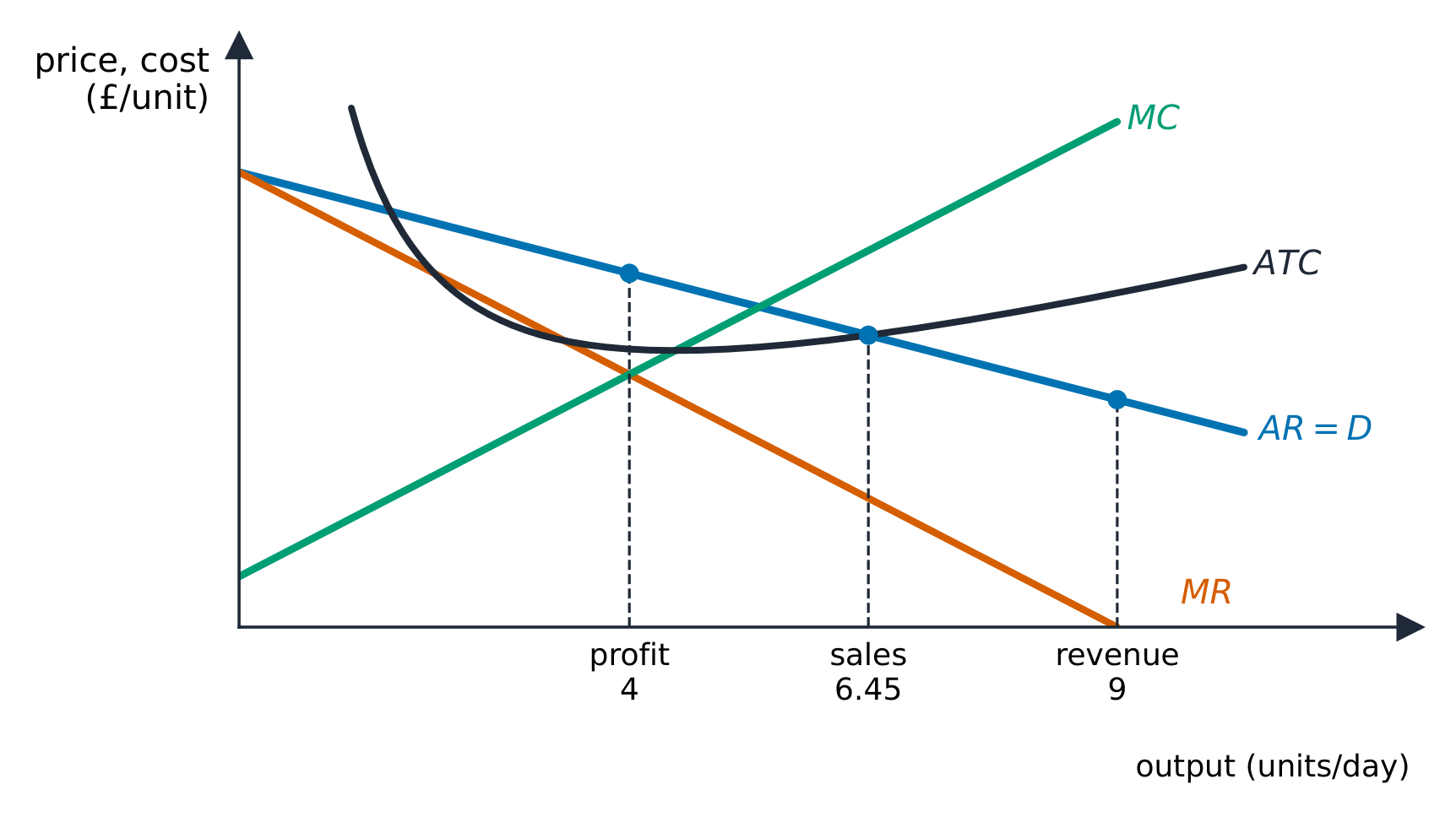
Syllabus
- explain alternative objectives of firms: profit maximisation, revenue maximisation, sales maximisation, satisficing
- explain the divorce of ownership from control (principal–agent problem) and its consequences
Source: Cambridge International syllabus
An objective is what the firm tries to achieve. A constraint limits the choices it can make. Profit, revenue and quantity sold are different measures. Compare them using the same demand, costs and period; do not infer an objective from one observed price alone.
Profit, revenue and sales: compare the same firm
Profit maximisation 利润最大化 means choosing the feasible output with the greatest total economic profit, including comparison with stopping production. For a smooth interior maximum, $MR=MC$ with marginal profit changing from positive to negative. An intersection alone does not prove a maximum; discrete outputs, capacity limits and several intersections require comparison of total profit.
Revenue maximisation 收益最大化 means choosing the greatest total revenue, $TR=PQ$, without subtracting costs. At a smooth interior revenue maximum, MR changes from positive to negative through zero. A price-taking firm with a positive fixed price has no such interior maximum: revenue rises until its feasible output limit. Revenue maximisation need not cover costs.
Sales maximisation 销售最大化 here means choosing the largest quantity subject to at least normal profit, so economic profit must be non-negative. In the standard continuous diagram, this is the largest feasible output where AR is at least ATC, often the higher-output AR=ATC intersection. The profit constraint is essential; the highest revenue and highest quantity are different objectives. Other stated constraints can change the answer.
Worked comparison. Reuse the illustrative monopoly model with daily demand $P=AR=18-Q$ and economic cost $TC=20+2Q+Q^2$. Prices/costs per unit are in pounds and Q is in units/day. The numerical coefficients have the compatible units. Then $TR=18Q-Q^2$ and $\pi=TR-TC=16Q-2Q^2-20$. Economic cost includes normal profit. This is a demand and cost model, not a claim about all firms.
| Q (units/day) | TR (£/day) | TC (£/day) | Profit (£/day) |
|---|---|---|---|
| 0 | 0 | 20 | −20 |
| 1 | 17 | 23 | −6 |
| 2 | 32 | 28 | 4 |
| 3 | 45 | 35 | 10 |
| 4 | 56 | 44 | 12 |
| 5 | 65 | 55 | 10 |
| 6 | 72 | 68 | 4 |
| 7 | 77 | 83 | −6 |
| 8 | 80 | 100 | −20 |
| 9 | 81 | 119 | −38 |
| 10 | 80 | 140 | −60 |
Among these feasible integer outputs, profit is greatest at Q=4, revenue at Q=9, and the largest quantity with non-negative profit is Q=6. At Q=0 the fixed cost remains; stopping gives −£20/day, below the £12/day maximum. Moving from Q=4 to Q=9 raises revenue by £25/day but cost by £75/day, so profit falls by £50/day.
$$\Delta TR=TR_9-TR_4=£81/\text{day}-£56/\text{day}=£25/\text{day}.$$
$$\Delta TC=TC_9-TC_4=£119/\text{day}-£44/\text{day}=£75/\text{day}.$$
$$\Delta\pi=\Delta TR-\Delta TC=£25/\text{day}-£75/\text{day}=-£50/\text{day}.$$
For a uniform-price seller, the price cut also affects earlier units. The extra five units bring in £45/day, but the original four each bring in £5 less, losing £20/day. Net revenue rises by £25/day. On a smooth diagram, the signed area under MR between the two outputs is the change in TR. A price-times-quantity rectangle gives total revenue at one output, not profit.
For divisible output in this model, profit maximisation gives $18-2Q=2+2Q$, so Q=4. Revenue maximisation gives $18-2Q=0$, so Q=9. The upper zero-profit boundary solves $16Q-2Q^2-20=0$, giving $Q=4+\sqrt{6}\approx6.45$ units/day. That is the continuous sales maximum subject to non-negative economic profit, rather than Q=6 from the integer table. Price is read from AR after choosing output. Do not round a continuous boundary upward to an infeasible integer output.
Profit satisficing and survival
Profit satisficing 满意化 means accepting a satisfactory profit target rather than the greatest possible profit. The target must be stated. In the integer table, a target of at least £10/day allows Q=3, 4 or 5. A manager who meets that target and then prefers the greatest quantity chooses Q=5, although Q=4 earns more profit. A different secondary aim could select another acceptable output. Satisficing does not mean every stakeholder must be happy or that all acceptable choices are equally good.
Survival means keeping the business operating, particularly when demand or access to finance is weak. A firm may cut investment or preserve cash while accepting a temporary economic loss. Profit and cash available to pay bills are different: a £200 monthly profit does not pay a bill if the customer has not yet paid. If only £1,200 is available and £1,500 must be paid now, the cash gap is £300. Borrowing or an agreed delay might bridge it, but neither is guaranteed. A temporary loss does not automatically imply immediate closure; compare future receipts with avoidable costs, cash needs and finance. Persisting indefinitely with avoidable losses does not establish a viable survival policy.
Objectives can change with ownership, competition, the economic climate and the time period. Owners and managers may disagree, as in the previous principal-agent example. A manager's revenue-linked bonus may encourage sales even when profit falls. Judge evidence about the stated target, constraints and behaviour rather than assuming every large firm follows one objective.
Limit pricing, predatory pricing and price leadership
Limit pricing 限制性定价 aims to discourage potential entrants. An established firm sets a price low enough to make entry unattractive, possibly sacrificing the higher short-run profit available at another price. The price need not be below the established firm's own cost. Predatory pricing 掠夺性定价 aims to force an existing rival out, using very low prices and potentially accepting short-run losses, with the intention of raising prices later to recover them. A low price or temporary loss alone does not establish that purpose: a promotion, falling costs or weak demand may also explain it.
Worked distinction. At the relevant output, an established firm's average cost is £4/unit and a potential entrant's expected average cost is £7/unit. A price of £6/unit leaves a £2/unit margin over the established firm's average cost but is £1/unit below the entrant's expected average cost. If used to deter entry, it is consistent with limit pricing. It may fail if the entrant lowers its costs, serves a different niche or expects prices to rise later. The cost estimates and the entrant's expectations matter; one observed price does not prove deterrence.
In a separate case, a firm charges £3/unit while its own average cost is £4/unit and an existing rival's is £5/unit at the relevant outputs. Both would make losses at those outputs. If the firm uses this to remove the rival and plans a later price rise to recoup losses, the strategy is consistent with predatory pricing. Success depends on finance, the rival's ability to survive and whether entry or re-entry prevents the later price rise. These illustrative costs do not prove the purpose or success of the strategy.
Price leadership 价格领导 means one firm sets or announces a price change and other firms follow. The leader may be a dominant firm or a firm regarded as a useful guide to market conditions. Following does not require a formal agreement. If a large supplier raises its price to £5 and others follow, the pattern is consistent with leadership; common input-cost changes could also explain similar prices. Evidence about timing, independent costs and communication is needed before claiming collusion. Leadership and entry deterrence describe different features of pricing and can coexist.
Demand elasticity and revenue on a normal demand curve
Price elasticity of demand 需求价格弹性 (PED) measures percentage quantity response divided by percentage price change. As in Topic 2, use the magnitude when classifying demand and distinguish point elasticity from a finite-change estimate. Revenue is $TR=PQ$, not profit.
For the illustrative straight-line demand $Q=18-P$, the gradient $\Delta Q/\Delta P=-1$ is constant. Point elasticity is $PED=(\Delta Q/\Delta P)(P/Q)$, so its magnitude varies along the line:
| P (£/unit) | Q (units/day) | PED magnitude | TR (£/day) |
|---|---|---|---|
| 14 | 4 | 3.5 | 56 |
| 9 | 9 | 1 | 81 |
| 6 | 12 | 0.5 | 72 |
At the elastic point, a small price cut raises revenue; in the inelastic part, a small price cut lowers it. Verify two finite changes directly rather than treating a point coefficient as an exact large-change forecast:
$$TR_{14}=P_{14}Q_{14}=(£14/\text{unit})(4\text{ units/day})=£56/\text{day}.$$
$$TR_{13}=P_{13}Q_{13}=(£13/\text{unit})(5\text{ units/day})=£65/\text{day}.$$
$$TR_6=P_6Q_6=(£6/\text{unit})(12\text{ units/day})=£72/\text{day}.$$
$$TR_5=P_5Q_5=(£5/\text{unit})(13\text{ units/day})=£65/\text{day}.$$
The midpoint P=9, Q=9 maximises revenue on this line. Unit point elasticity identifies that point; it does not mean revenue is unchanged over every finite movement away from it. Revenue is constant along a whole unit-elastic demand segment, which is a different statement. Revenue changes alone do not establish profit changes without costs.
Kinked demand: specify how rivals react
A kinked demand curve 拐折需求曲线 models a firm expecting rivals to ignore a price rise but match a price cut. Above the current price, buyers can switch to rivals, making demand relatively elastic. Below it, matching cuts limit the extra buyers gained, making demand relatively inelastic. These are assumptions about reactions, not a rule for every oligopoly.
Illustrative model. At the kink, P=£10/unit and Q=10 units/day. Above that price, inverse demand is $P=15-0.5Q$ for Q up to 10. Below it, $P=30-2Q$ for Q from 10 to 15. The coefficients use compatible units. At the kink the upper and lower one-sided PED magnitudes are 2 and 0.5 respectively; the point at the kink itself has no single slope.
A rise to £11/unit gives Q=8, so TR falls from £100/day to £88/day. A cut to £9/unit gives Q=10.5, so TR falls to £94.50/day. The smaller quantity response below the kink does not mean quantity fails to rise; it rises too little to offset the lower price.
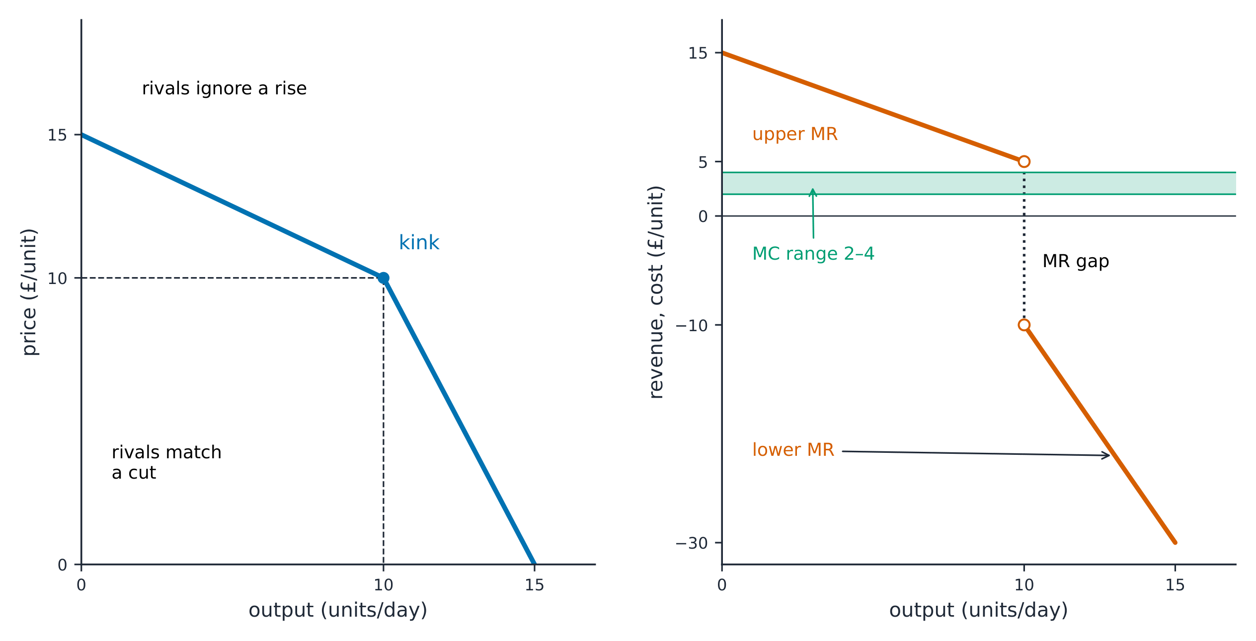
The two marginal-revenue branches are $MR=15-Q$ above the kink and $MR=30-4Q$ below it. At Q=10 the gap extends from −£10 to £5/unit. If constant MC changes from £2 to £4/unit, both lie inside it: reducing output loses revenue greater than saved cost, while expanding adds cost greater than revenue. The profit-maximising output remains 10 and price remains £10/unit.
With fixed cost £10/day, the profit calculation changes even though price and output do not:
$$TC_2=F+MC_2Q=£10/\text{day}+(£2/\text{unit})(10\text{ units/day})=£30/\text{day}.$$
$$\pi_2=TR-TC_2=£100/\text{day}-£30/\text{day}=£70/\text{day}.$$
$$TC_4=F+MC_4Q=£10/\text{day}+(£4/\text{unit})(10\text{ units/day})=£50/\text{day}.$$
$$\pi_4=TR-TC_4=£100/\text{day}-£50/\text{day}=£50/\text{day}.$$
This rigidity result has limits. At MC=£6/unit, above the gap, the best output becomes Q=9 and price £10.50/unit in this same model. Rival reactions, demand and costs can also change. The kinked-demand model illustrates why an existing price might persist over a range of costs; it does not explain how the initial price was chosen or prove collusion.
Explore
Firm objective lab
Classify real firm decisions by the objective they reveal.
Vocabulary
Train
| English |
|---|
| profit maximisation/ˈprɒfɪt ˌmæksɪmaɪˈzeɪʃn/ |
| revenue maximisation/ˈrevənjuː ˌmæksɪmaɪˈzeɪʃn/ |
| sales maximisation/seɪlz ˌmæksɪmaɪˈzeɪʃn/ |
| satisficing/ˈsætɪsfɪsɪŋ/ |
| limit pricing/ˈlɪmɪt ˈpraɪsɪŋ/ |
| predatory pricing/ˈpredətəri ˈpraɪsɪŋ/ |
| price leadership/praɪs ˈliːdəʃɪp/ |
| price elasticity of demand/praɪs ɪlæˈstɪsɪti ɒv dɪˈmænd/ |
| kinked demand curve/kɪŋkt dɪˈmænd kɜːv/ |
7.8
Exam tips
- Identify the measure and constraint before choosing an output. Compute TR, TC and profit separately; more sales or revenue does not necessarily mean more profit.
- Use MR=MC as a conditional marginal test and compare feasible alternatives, boundaries and stopping. Read price from AR at the chosen Q, not from MR or MC.
- On a standard smooth U-shaped cost diagram, MC crosses AC at its interior minimum because MC below AC lowers AC and MC above AC raises it. This is not a universal shape for every technology or discrete table.
- Distinguish market structures by entry/exit, product differences, information and price-setting power as well as firm numbers. Normal profit means economic cost is covered, not that revenue is zero.
Vocabulary card meanings
Pareto optimality: A situation in which nobody can gain unless someone else loses. dynamic efficiency: Improvement over time through new products and better methods. factor immobility: When land, labour, or capital cannot easily move to a better use. private benefit: The gain kept by the person who takes an action. social benefit: The gain to society, including gains to people who did not pay. marginal analysis: Comparing the extra cost and extra gain of one more unit. perfect competition: A market with many firms, an identical product, and free entry. price competition: Rivalry that tries to win buyers by charging less. horizontal integration: Joining with a firm at the same stage of production. vertical integration: Joining with a firm at another stage of the same chain. conglomerate integration: Joining with a firm in an unrelated industry. barriers to exit: Costs that make it hard for a firm to leave an industry. revenue maximisation: Choosing the output that brings in the largest sales income. sales maximisation: Choosing the output that brings in the most sales income while profit stays at or above a required minimum. divorce of ownership from control: Shareholders own the firm, but hired managers run it. marginal external cost: The extra cost one more unit imposes on other people. marginal external benefit: The extra gain one more unit gives to other people. moral hazard: Taking bigger risks because someone else will bear the loss. increasing returns to scale: Output rises by a larger percentage than all of the inputs. decreasing returns to scale: Output rises by a smaller percentage than all of the inputs. minimum efficient scale: The smallest output at which long-run average cost is lowest. internal economies of scale: Lower average cost that a firm gains by growing itself. external economies of scale: Lower average cost that a firm gains because its industry grows. internal diseconomies of scale: Higher average cost as one firm becomes too large to manage. external diseconomies of scale: Higher average cost as the surrounding industry grows too crowded. X-inefficiency: Extra cost because a sheltered firm does not work to cut waste. contestable market: A market that new firms can enter and leave at low cost. Prisoner's Dilemma: A game in which each side's safe choice leaves both worse off. backward vertical integration: Taking over a supplier at an earlier stage of the chain. forward vertical integration: Taking over a customer at a later stage, such as a retailer. first-degree price discrimination: Charging each buyer the highest price that buyer will pay. second-degree price discrimination: Charging different prices for different amounts bought. third-degree price discrimination: Charging different groups of buyers different prices. limit pricing: Setting a low enough price to keep a new rival out. predatory pricing: Pricing below cost in order to drive a rival out. price leadership: One firm sets the price and the other firms follow it. kinked demand curve: Demand that is flatter above the current price and steeper below it.
Interactive lessons on this topic
Work through it step by step, with instant-check exercises.