This topic looks at how governments correct market failure 市场失灵, make incomes fairer, and act in the labour market.
Government microeconomic intervention (A Level)
A-Level Economics · Topic 8
 8:20
8:20
Government microeconomic intervention (A Level)
Three ordinary pictures. Cigarettes, sold cheaply to anyone who wants them. A hillside of tin roofs, looking down on a rich city district. A factory floor…
English narration · English + 中文 subtitles burned in
8.1
Correcting market failure
Syllabus
- explain policies to correct market failure: taxes, subsidies, price controls, tradable permits, regulation, provision, nationalisation and privatisation
- explain competition policy and the concept of government failure
Source: Cambridge International syllabus
Start with the cause of market failure and the outcome being targeted. Reducing a quantity, raising revenue and improving resource allocation are different aims. This unit builds on the private/social cost and benefit diagrams in the earlier A-Level microeconomics topic; a policy answer must use those diagrams, not just name a tool.
Congestion: identify harm to other people
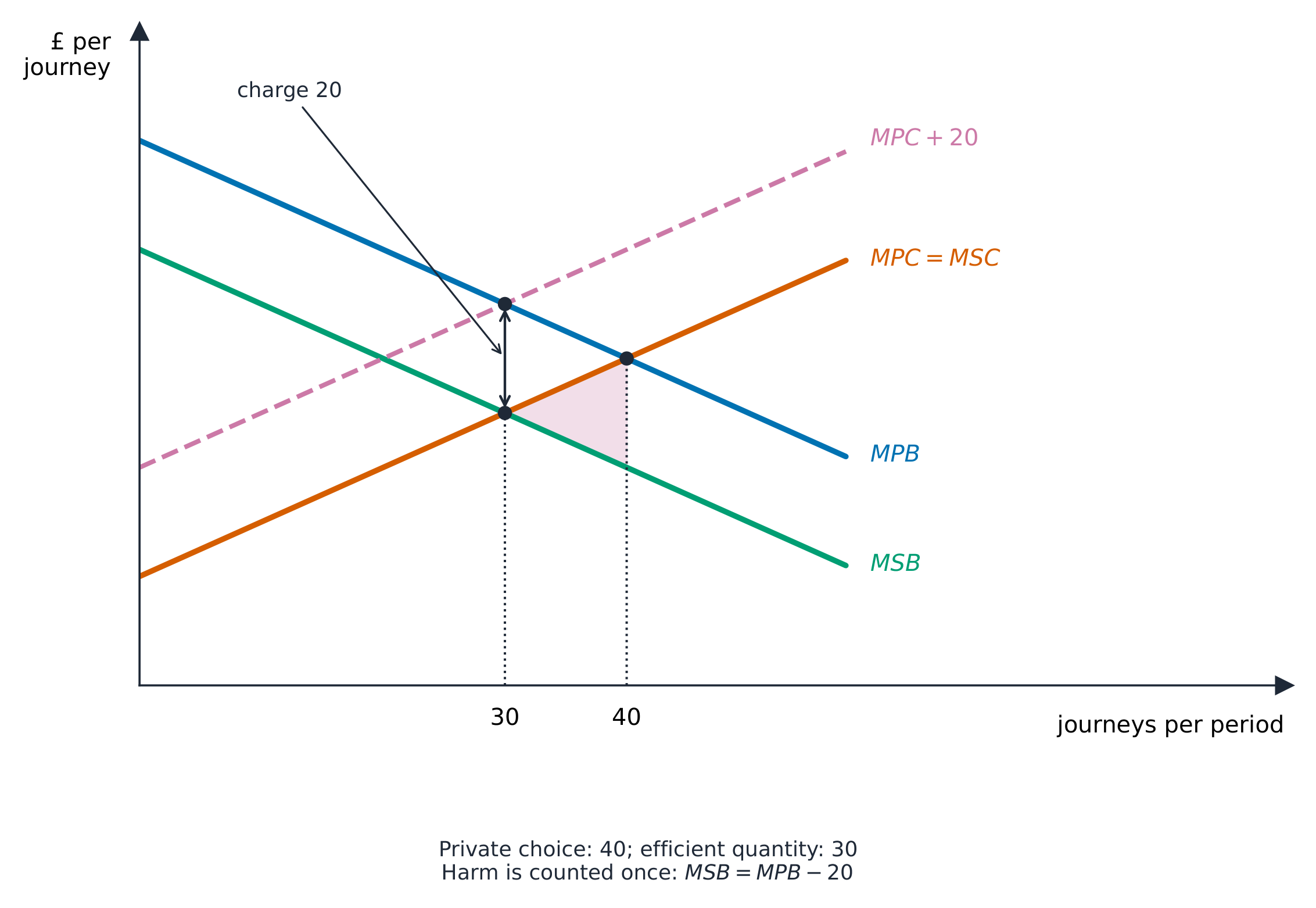
A driver considers their own journey benefit and private costs. An extra trip can also delay other road users. That extra delay is an external harm; it is different from the driver's own time cost. In a negative consumption-externality diagram, marginal social benefit is below marginal private benefit. Alternatively the extra harm can be represented on the cost side, but do not subtract it from benefits and add it to costs in the same calculation.
Worked illustrative model. Quantity Q is journeys per period; all marginal benefits and costs are in pounds per journey. Marginal private benefit is MPB =100 −Q. Marginal private cost is MPC =20 +Q. External harm is £20 per journey. In the benefit-side diagram, MSB =80 −Q and MSC =MPC. These are constructed values, not estimates of a real city's optimal charge. The private outcome ignores harm to others:
$$MPB=MPC\quad\Rightarrow\quad 100-Q=20+Q$$
$$Q_m=(100-20)/2=40\text{ journeys per period}$$
$$C_m=20+Q_m=20+40=\text{£}60\text{ per journey}$$
The efficient quantity balances marginal social benefit and cost:
$$MSB=MSC\quad\Rightarrow\quad 80-Q=20+Q$$
$$Q^*=(80-20)/2=30\text{ journeys per period}$$
$$C^*=20+Q^*=20+30=\text{£}50\text{ per journey}$$
For journeys between 30 and 40, marginal social cost exceeds marginal social benefit. Removing these trips avoids a triangular deadweight loss:
$$DWL=\tfrac 12(Q_m-Q^*)\,MEC=\tfrac 12(40-30)(20)=\text{£}100\text{ per period}$$
A charge: follow incentives, output and revenue
An indirect tax 间接税 or road-use charge raises the private marginal cost faced by the traveller. In this model a specific £20 charge gives:
$$MPB=MPC+t\quad\Rightarrow\quad 100-Q=20+Q+20$$
$$Q_t=(100-40)/2=30\text{ journeys per period}$$
$$C_{\rm faced}=MPC(Q_t)+t=20+30+20=\text{£}70\text{ per journey}$$
$$R=tQ_t=20(30)=\text{£}600\text{ per period}$$
The £70 is the traveller's marginal private journey cost including the charge; £50 is private cost excluding it. Costs may include time as well as money, so do not describe these numbers as a fare and a transport company's cash receipts. Tax revenue must not be counted as an additional social loss: it is transferred to government. External harm from the remaining 30 journeys is still £600; efficient output does not mean zero harm. The aim is to remove trips whose social cost exceeds their social benefit, not necessarily to ban all travel.
The corrective charge equals marginal external harm at the efficient quantity under this model's assumptions. With varying harm, different times, incomplete coverage, market power or uncertain behaviour, a uniform charge need not be exactly efficient. Diversion to another road may move harm rather than remove it. Assess monitoring, collection costs, distributional effects, availability of alternatives and how revenue is used.
A specific tax is a fixed amount per unit. An ad valorem tax 从价税 is a proportion of a taxable price: at a 20% rate the tax on a £50 taxable price is £10, while on £80 it is £16. Neither the rate nor revenue alone establishes that the tax matches external harm.
Subsidising an alternative is a different mechanism
A subsidy 补贴 can make public transport cheaper or support additional capacity. It reduces road congestion only to the extent that it changes relevant travel choices; not every additional passenger was previously a car user.
Separate transport-market example. Bus demand is P =50 −Q and original supply is P =10 +Q, with pounds per trip and trips per period. Before subsidy, Q 20/P 30. A per-trip producer subsidy £10 gives buyer-facing supply P =Q:
$$P_D=P_S-s\quad\Rightarrow\quad 50-Q=10+Q-10$$
$$Q_1=50/2=25\text{ bus trips per period}$$
$$P_b=50-Q_1=50-25=\text{£}25\text{ per trip}$$
$$P_s=P_b+s=25+10=\text{£}35\text{ per trip}$$
$$G=sQ_1=10(25)=\text{£}250\text{ per period}$$
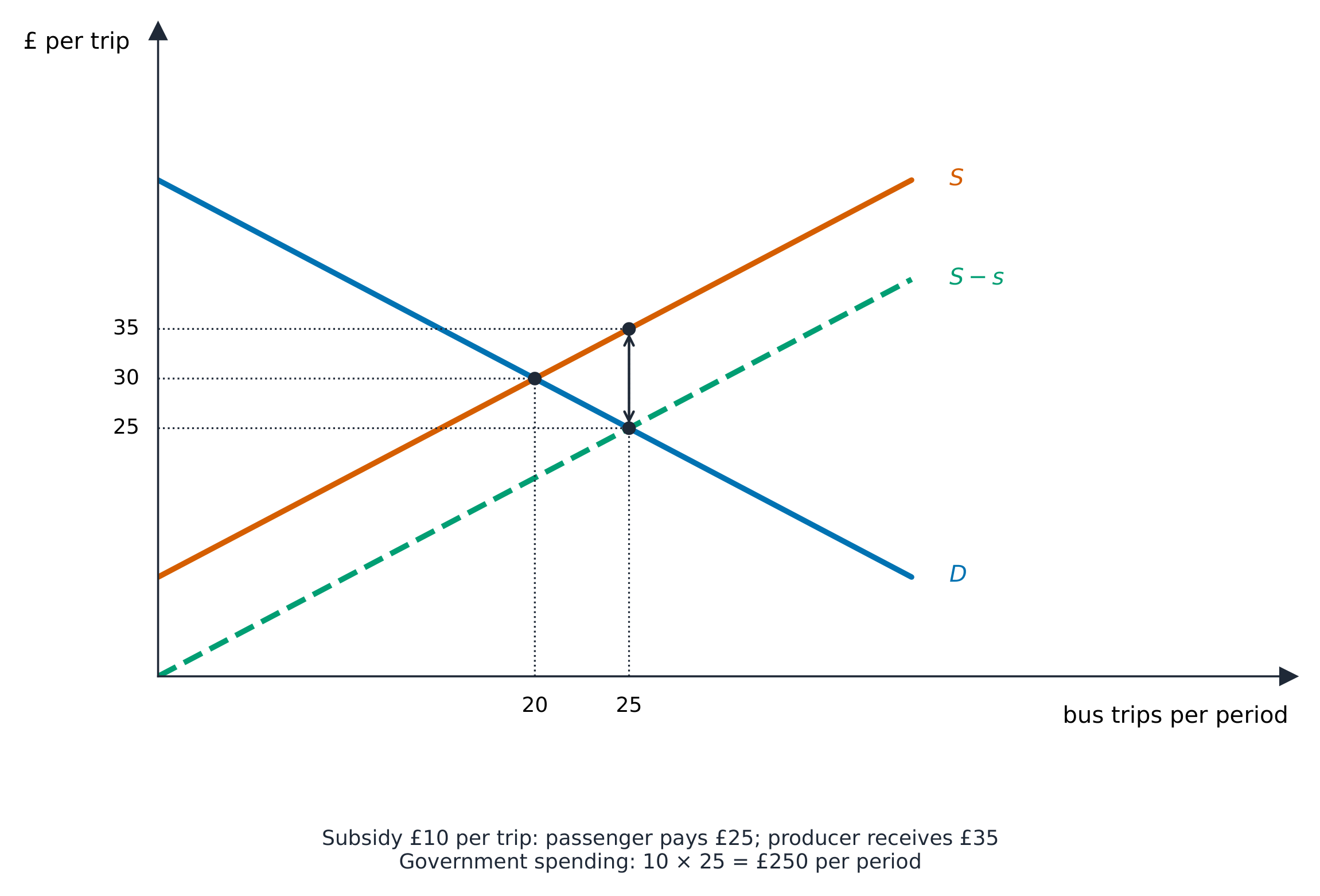
The five extra bus trips do not establish five fewer car trips. Some passengers may switch from walking, and the routes or times may not serve congested journeys. Compare a road charge with this subsidy using price responses, substitution, service quality and fiscal opportunity cost. A subsidy also does not create new buses or staff immediately when capacity is fixed.
Price controls: distinguish affordability from allocation
A price control 价格管制 sets a legal ceiling or floor. In a separate competitive market, demand is Qd =30 −P and supply Qs =P. Original equilibrium is P 15/Q 15. A ceiling 12 gives demand 18 but supply 12: a shortage 6, with only 12 units supplied legally without another source. A lower posted price does not establish better availability or efficient allocation. In a market with power or a different supply structure, first identify the relevant model; do not assume every ceiling has the same effects. Minimum wages below provide a further price-floor application.
Quantity rules, permits and property rights
Regulation 管制 can impose standards or restrictions. A production quota 生产配额 limits a stated quantity; a prohibition 禁令 bans a stated activity; a licence 许可证 sets conditions for legal participation. A cap can make the allowed quantity clear, but enforcement, exemptions and illegal activity determine the actual outcome. Different rules work through different channels; not all regulation is simply a quantity limit.
Tradable permits 可交易许可证 combine an overall emissions cap with trade in permission to emit. Suppose two firms would otherwise emit two units each. A cap of two units requires two reductions overall. Each of A's two possible reductions costs £10; each of B's costs £30. Making each cut one costs £40. Allowing A to cut two and B none costs £20 and meets the same cap. A permit trade can reward these cheaper reductions. This least-cost argument assumes the emissions are comparable, trades are feasible and compliance is monitored; local hotspots, market power or poor enforcement can change the result. A permit price is a transfer between traders, not another resource cost of abatement.
Clear property rights 产权 may let affected parties negotiate. If reducing a factory's noise costs £80 and benefits a neighbouring household by £120, there is a possible gain of £40 to share through agreement. Bargaining can be difficult when thousands of people are affected, harm is hard to measure, rights are unclear or enforcing agreement is costly. This is a conditional alternative to a direct tax or ban, not proof that all externalities solve themselves.
Information, nudges, provision and ownership
State provision 政府提供 means government supplies or arranges a service; it need not be free. Extra buses or safer cycling routes may address an actual missing alternative. Information about routes or travel times may help where people lack knowledge, but cannot by itself supply a bus that does not exist. A nudge 轻推 changes how a choice is presented while leaving options available, such as making a public-transport route the default suggestion. Its effect depends on the cause of behaviour and whether travellers can use the suggested option.
Nationalisation 国有化 transfers ownership into the public sector; privatisation 私有化 transfers it to private owners. Neither change alone removes monopoly power, creates a third-party price or ensures adequate capacity. Compare objectives, incentives, regulation, investment and accountability before predicting the outcome.
Competition policy and government failure
Competition policy 竞争政策 addresses practices or structures that weaken effective competition. A firm with monopoly power 垄断势力 may restrict output and raise price. Preventing price-fixing, reviewing mergers or reducing entry barriers can help, but a large size alone does not establish harmful behaviour. Merger cost savings must be compared with effects on rivalry and customers; regulation of a natural monopoly must consider costs, quality and investment.
Government failure 政府失灵 means intervention produces worse resource allocation than the relevant alternative. A policy being costly, imperfect or unpopular is not enough to establish failure. Compare benefits with administration, compliance and opportunity costs. Poor estimates of harm, weak enforcement, time lags, unintended diversion or decisions serving a narrow group can reduce the gain.
Deregulation 放松管制 removes or relaxes a restriction. Suppose an exclusive route licence blocks other bus operators. Allowing entry may increase choice and rivalry, but entry is not guaranteed if depot access or scale remain barriers. Retaining safety standards and managing scarce road space may still be needed. Removing a rule does not by itself remove congestion or establish a welfare gain. Compare benefits from entry with service quality, coverage and external costs.
Build a two-policy judgement. For congestion, explain the external harm and inefficient quantity with a labelled diagram. Show how a charge changes private incentives; compare it with an alternative-transport subsidy or direct provision. Evaluate responsiveness, routes and capacity, time, costs and who is affected. A justified combination may work better than either policy alone, but must be assessed against feasible alternatives. In a climate-change question also consider cross-border effects, coordination, bargaining or private action; do not conclude that all government intervention succeeds or that government is the only possible source of improvement.

Explore
A private-market charge shift
Explore how an extra cost changes private equilibrium. This display does not show social-benefit curves, efficient quantity or welfare loss; use the handout diagram for those.
Vocabulary
Train
| English |
|---|
| market failure/ˈmɑːkɪt ˈfeɪlɪə/ |
| indirect tax/ɪndaɪˈrekt tæks/ |
| subsidy/ˈsʌbsɪdi/ |
| price control/praɪs kənˈtrəʊl/ |
| tradable permits/ˈtreɪdəbl ˈpɜːmɪts/ |
| regulation/ˌreɡjʊˈleɪʃn/ |
| state provision/steɪt prəˈvɪʒn/ |
| nationalisation/ˌnæʃənəlaɪˈzeɪʃn/ |
| privatisation/ˌpraɪvətaɪˈzeɪʃn/ |
| monopoly power/məˈnɒpəli ˈpaʊə/ |
| competition policy/ˌkɒmpəˈtɪʃn ˈpɒlɪsi/ |
| government failure/ˈɡʌvənmənt ˈfeɪlɪə/ |
| ad valorem tax/æd ˈvælɒrəm tæks/ |
| production quota/prəˈdʌkʃn ˈkwəʊtə/ |
| prohibition/prəhɪˈbɪʃn/ |
| licence/ˈlaɪsəns/ |
| property rights/ˈprɒpəti raɪts/ |
| nudge/nʌdʒ/ |
| deregulation/diːˌreɡjʊˈleɪʃn/ |
8.2
Equity and redistribution

Syllabus
- distinguish equity, equality, and the difference between income and wealth
- explain the Lorenz curve and Gini coefficient and policies to redistribute income and wealth (taxation, benefits, the difficulty of redistributing wealth)
Source: Cambridge International syllabus
Equity 公平 means fairness; equality 平等 means equal amounts, treatment or opportunities, depending on the comparison. People may disagree about what is fair. Two households each receive £100: equal cash amounts, but not necessarily equal opportunities if one needs costly disability support. Allocative efficiency concerns whether resources produce the greatest net social benefit. An efficient allocation can still be judged unfair. Better access to education may improve both fairness and efficiency; neither a conflict nor a joint gain is automatic.
Inequality 不平等 describes differences in a distribution. Income 收入 is a flow over a period. Wealth 财富 is a stock of assets less relevant debts at a date. A person earning £2000 per month with a £150000 home and £100000 mortgage has £50000 net housing wealth, before other assets and debts. Monthly income and this stock cannot be added as if they had the same units.

Measuring inequality
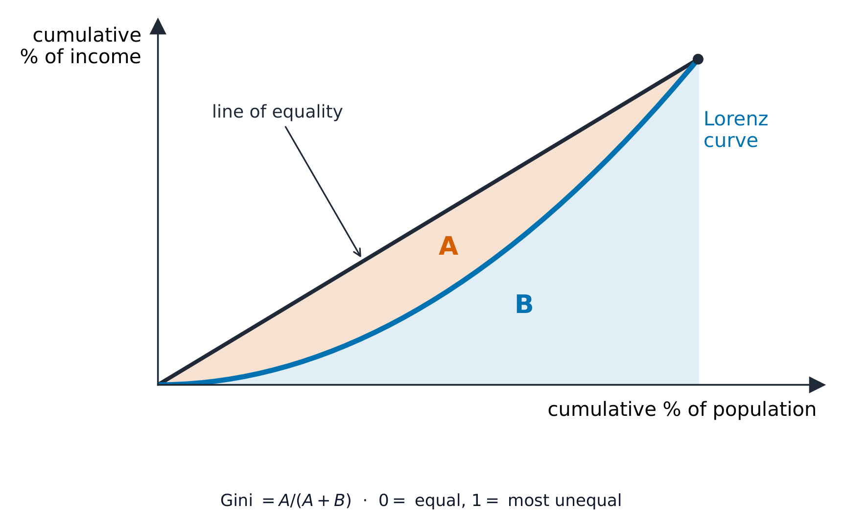
A Lorenz curve 洛伦兹曲线 plots cumulative income share vertically against cumulative population share horizontally, ordering people from poorest to richest. Both axes run from 0 to 100%. The diagonal represents equal shares. Let A be the area between the diagonal and the curve, and B the area below the curve. The Gini coefficient 基尼系数 is:
$$G=\frac{A}{A+B}$$
Zero represents perfect equality; values nearer one indicate greater measured inequality. Use the same population, income definition and period when comparing. Income and wealth Ginis describe different distributions. A Gini does not establish absolute living standards, the cause of a change or the position of every group.
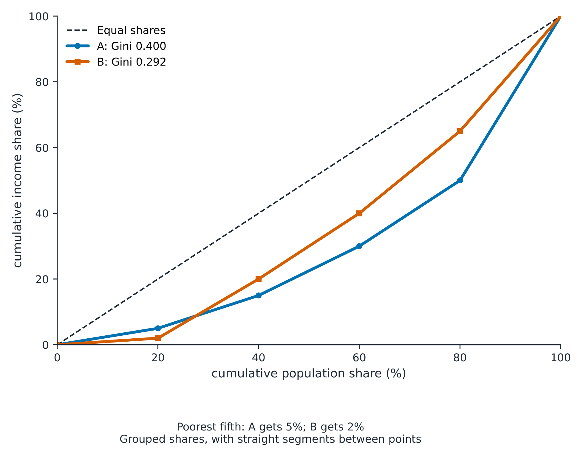
Worked data comparison. Each row below is one fifth of the population, ordered by income within that economy. Entries are shares of total income, not pounds.
| Fifth, poorest first | A share % | B share % |
|---|---|---|
| 1 | 5 | 2 |
| 2 | 10 | 18 |
| 3 | 15 | 20 |
| 4 | 20 | 25 |
| 5 | 50 | 35 |
Add the shares: A's cumulative percentages are 0, 5, 15, 30, 50, 100; B's are 0, 2, 20, 40, 65, 100. Their Lorenz curves cross. For straight segments between these grouped points, the illustrative Ginis are 0.400 and 0.292. B has a lower overall Gini but its poorest fifth receives a smaller share, 2% rather than 5%. A lower Gini alone cannot prove that one Lorenz curve lies everywhere above another. Nor do these percentages establish which poorest group has more pounds without total income and population information.
Poverty and the poverty trap
Absolute poverty 绝对贫困 means resources fall below a specified basic-needs standard. Relative poverty 相对贫困 means resources fall below a specified standard relative to society, often a fraction of median income. State the measure and household adjustment. A relative threshold may rise as median income rises. A Gini can fall while some people remain unable to afford basic needs.
A poverty trap 贫困陷阱 can arise when extra earnings bring higher taxes and withdrawal of benefits, leaving little extra disposable income and weakening the financial return to work. It is not simply another name for low income.
Worked example, pounds per week. Earnings rise from 100 to 150; tax rises from 0 to 20; benefits fall from 80 to 55.
$$Y_d=Y-T+B$$
$$Y_{d0}=100-0+80=\text{£}180\text{ per week}$$
$$Y_{d1}=150-20+55=\text{£}185\text{ per week}$$
Of £50 extra earnings, only £5 remains. The combined effective marginal withdrawal rate is:
$$m=\frac{\Delta T-\Delta B}{\Delta Y}=\frac{20-(-25)}{50}=0.90=90\%$$
Travel or childcare costs may further change the gain. The calculation identifies a financial incentive, not a guarantee about an individual's decision. Education, health and care responsibilities also matter.
Policies to redistribute
A progressive tax 累进税 takes a larger average share of higher incomes. Benefits 福利金 paid without a current production exchange are transfer payments 转移支付. Taxes, transfers and services can change disposable income and opportunity; this is redistribution 再分配. They may also change work, saving and investment incentives. Wealth policies require attention to valuation, liquidity, enforcement and avoidance; income taxes have their own enforcement problems. Which is easier to administer depends on the actual tax base and institutions.

A negative income tax 负所得税 pays a net transfer below a break-even income and collects net tax above it. In an illustrative weekly rule, net tax T = 0.5Y − 80. Negative T means a payment to the household, not a debt it owes.
| Earnings Y | Net tax T | Disposable Y − T |
|---|---|---|
| 0 | −80 | 80 |
| 100 | −30 | 130 |
| 160 | 0 | 160 |
| 200 | 20 | 180 |
For example, $T=0.5(100)-80=-\text{£}30$ and $Y_d=100-(-30)=\text{£}130$ per week. Each extra pound of earnings adds 50p to disposable income in this rule before other taxes, transfers or costs. Assess adequacy, finance, take-up and administration; a smooth withdrawal does not eliminate every barrier to employment.
Universal benefits 普惠福利 go to everyone within a defined eligible category, such as all eligible children. Means-tested benefits 经济状况审查福利 depend on income or assets. A universal basic income 全民基本收入 is a regular unconditional payment to every individual in the defined population. A child benefit is not automatically a UBI.
Comparison task. A category contains 100 households; 40 meet a low-income test. A payment of £80 per household costs £8000 if universal within the category or £3200 if limited to the 40, before administration and tax recovery. The smaller gross payment bill does not prove greater net benefit: check exclusions, take-up, withdrawal incentives and administrative costs. Universal payments may reach households with high incomes but the tax system can recover some cost. Accessible education and health services may improve opportunity, yet places, quality and financing constrain the result. Defend a policy against a feasible alternative, addressing both distribution and efficiency.
Explore
Inequality policy route
Follow how policy can change disposable income and opportunity.
Explore
Bend the Lorenz curve
Explore this family of generated income shares. The tool does not establish that arbitrary Gini rankings imply pointwise Lorenz dominance; use the handout crossing-curves example.
Vocabulary
Train
| English |
|---|
| equity/ˈekwɪti/ |
| equality/iːˈkwɒlɪti/ |
| inequality/ɪniːˈkwɒlɪti/ |
| income/ˈɪŋkʌm/ |
| wealth/welθ/ |
| Lorenz curve/ˈlɒrənts kɜːv/ |
| Gini coefficient/ˈdʒiːni ˌkəʊɪˈfɪʃənt/ |
| progressive tax/prəˈɡresɪv tæks/ |
| benefits/ˈbenɪfɪts/ |
| transfer payments/ˈtrænsfɜː ˈpeɪmənts/ |
| redistribution/ˌriːˌdɪstrɪˈbjuːʃn/ |
| absolute poverty/ˈæbsəluːt ˈpɒvəti/ |
| relative poverty/ˈrelətɪv ˈpɒvəti/ |
| poverty trap/ˈpɒvəti træp/ |
| negative income tax/ˈneɡətɪv ˈɪŋkʌm tæks/ |
| universal benefits/ˌjuːnɪˈvɜːsl ˈbenɪfɪts/ |
| means-tested benefits/miːnz ˈtestɪd ˈbenɪfɪts/ |
| universal basic income/ˌjuːnɪˈvɜːsl ˈbeɪsɪk ˈɪŋkʌm/ |
8.3
Labour markets

Syllabus
- explain the demand for and supply of labour, marginal revenue product (MRP) and wage determination in competitive labour markets
- explain monopsony, trade unions, the national minimum wage, wage differentials and discrimination, and government intervention
Source: Cambridge International syllabus
In a labour market 劳动力市场 workers offer labour and employers hire it. State the occupation, location and period. A wage 工资 is a payment rate, not the number of workers. Distinguish the whole occupation's market from one small employer taking its wage as given.
The demand for labour
The demand for labour 劳动力需求 is a derived demand 派生需求: demand for the product affects demand for the workers who make it. The marginal revenue product 边际收益产品, MRP, is the extra revenue from an extra worker-hour:
$$MRP=MPP\times MR$$
MPP is marginal physical product; MR is the extra revenue per unit of output. If the firm sells output at a constant competitive price P, MR = P and the shortcut MRP = MPP × P applies. An extra worker producing 3 units per hour sold at a constant £6 per unit brings £18 extra revenue per hour. If relevant marginal revenue is £4 instead, MRP is £12, not £18. Hiring compares MRP with marginal employment cost; only a wage-taking employer with no extra employment costs can use the wage directly.
Whole-worker decision. Extra hourly revenues from workers 1–5 are £28, £24, £18, £12 and £8. With a fixed hourly wage of £14 and no other changing costs, hire three: worker 3 adds £4 net revenue, worker 4 subtracts £2. Exact MRP = wage equality need not occur with whole workers. In a smooth divisible-labour model, an interior maximum uses MRP = marginal employment cost.
Market and firm supply are different
The supply of labour 劳动力供给 to an occupation depends on wages, training, population, migration, mobility, working conditions and alternatives. A wage change gives a movement along the given curve; training or migration can shift it. An individual worker's hours need not rise at every wage: income and substitution effects can pull in different directions. The upward market curve below is an explicit model assumption.
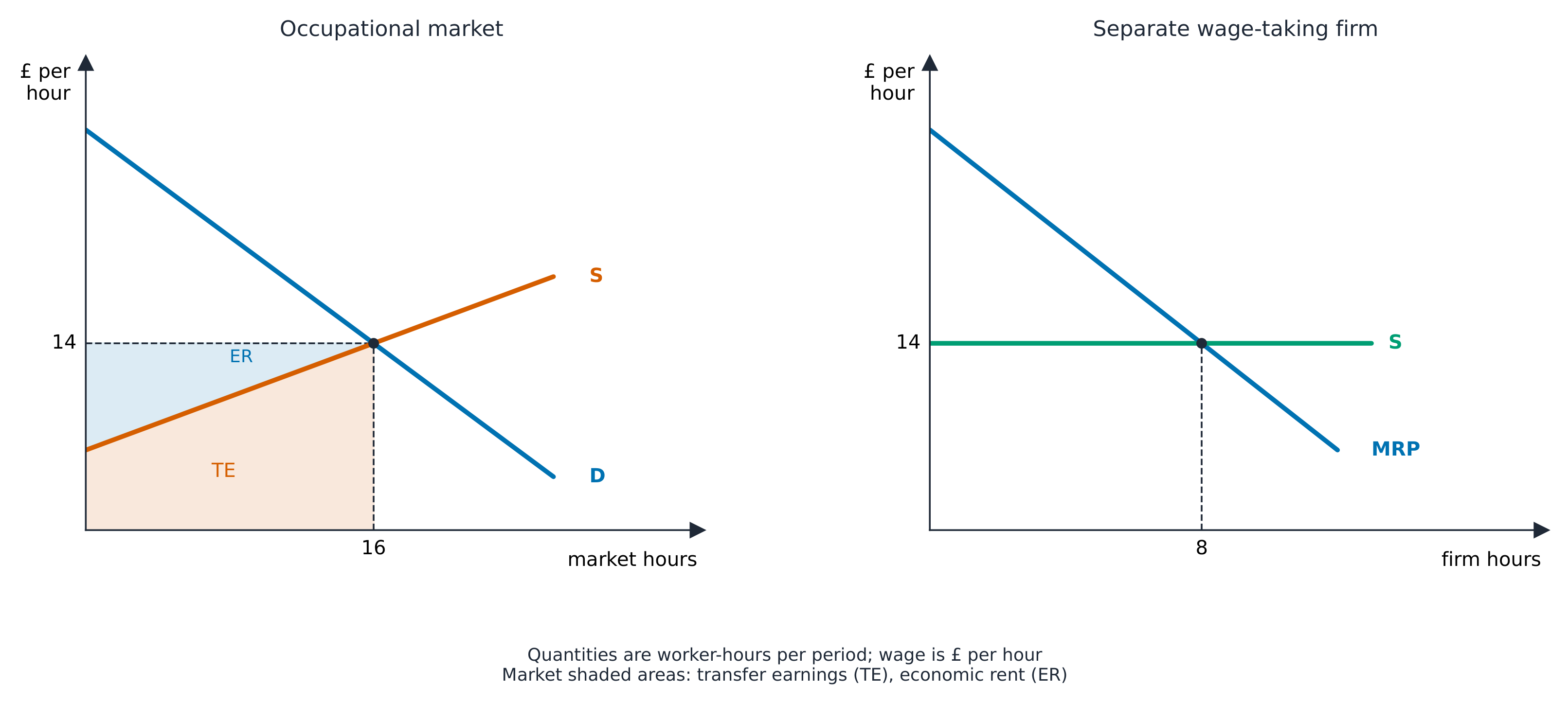
Market illustration. In pounds per hour and worker-hours per period, demand is $w=30-L$ and supply $w=6+0.5L$. At equilibrium:
$$D=S\quad\Rightarrow\quad30-L=6+0.5L$$
$$L^*=\frac{30-6}{1.5}=16\text{ worker-hours per period}$$
$$w^*=6+0.5L^*=6+0.5(16)=\text{£}14\text{ per hour}$$
Separate small-firm illustration. One wage-taking firm has $MRP=30-2l$ and can hire at £14 per hour without changing that market wage. Its supply curve is horizontal at 14 even though market supply slopes upward.
$$\begin{aligned}
MRP=w&\quad\Rightarrow\quad30-2l=14\\
l^*&=\frac{30-14}{2}=8\text{ firm worker-hours per period}
\end{aligned}$$
These are separate illustrations, not an exact aggregation of identical firms. A productivity increase at this firm alone shifts its MRP to $34-2l$, giving $l=(34-14)/2=10$ with wage still 14. A separate market-wide demand shift to $w=36-L$, holding market supply fixed, gives $L=(36-6)/1.5=20$ and wage $6+0.5(20)=16$. A perfectly elastic supply to a firm does not mean the market wage can never change.
Labour-saving machinery can substitute for labour but lower costs and expand output. Evaluate the net demand change rather than treating any new machine as a certain fall in employment. Better working conditions or easier qualification may attract workers at a given wage; increased product demand shifts MRP, while a change in wage alone moves along the given demand curve.
When the market is not competitive
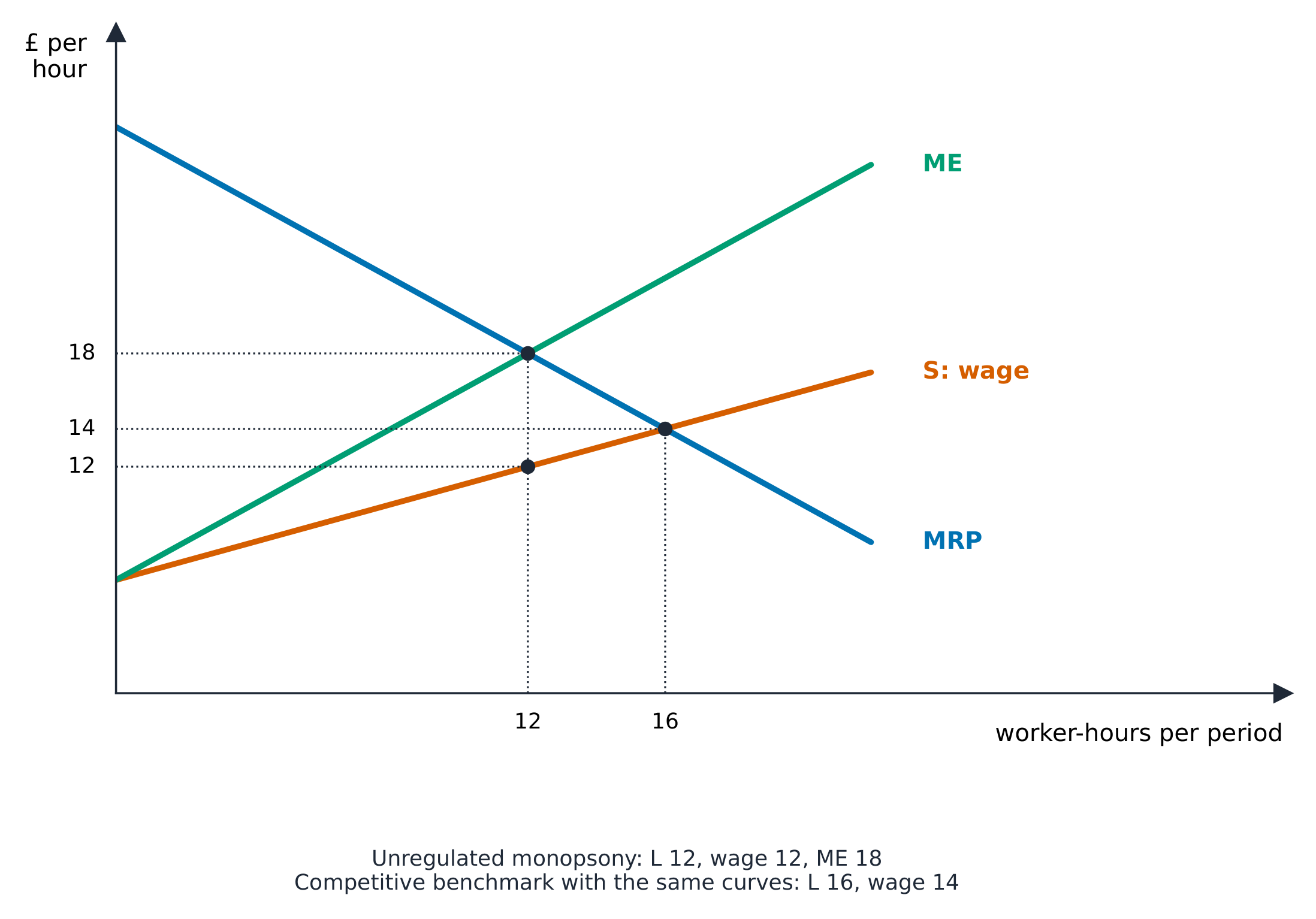
A monopsony 买方垄断 employer faces upward-sloping labour supply. In a uniform-wage model, hiring more workers requires raising the wage for existing workers too, so marginal employment cost ME exceeds the wage. Use a separate local-market example with MRP = 30 − L and wage supply w = 6 + 0.5L. Total wage cost is $TC_L=wL=6L+0.5L^2$, so $ME=6+L$.
$$\begin{aligned}
MRP=ME&\quad\Rightarrow\quad30-L=6+L\\
L_m&=\frac{30-6}{2}=12\text{ worker-hours per period}\\
w_m&=6+0.5L_m=6+0.5(12)=\text{£}12\text{ per hour}\\
ME_m&=6+L_m=6+12=\text{£}18\text{ per extra worker-hour}
\end{aligned}$$
Choose quantity using MRP = ME, then read wage from supply. Paying 18 to everyone would be the wrong wage. Holding the same MRP and supply curves fixed, the competitive benchmark is L = 16 and w = 14. This comparison depends on the uniform-wage model and the stated curves.
A national minimum wage 全国最低工资 is a legal floor for covered workers. In the competitive market above, floor 20 gives labour demand 10 and supply 28: excess supply 18 worker-hours, with employment 10 in the simple model. A floor below 14 is not binding there. Compliance, coverage, hours, productivity, enforcement and demand elasticity affect actual outcomes. Excess supply in the model is not a complete measure of a country's recorded unemployment.
Monopsony floors. In the monopsony example, a floor of 14 makes marginal employment cost 14 while up to 16 worker-hours are available at that wage. Hiring expands to 16, where MRP = 14. Above 16 the employer must raise the uniform wage and marginal cost jumps above 14. A higher floor of 20 instead gives demand 10 and available supply 28, so the employer hires 10, below its original 12. A wage floor can raise both wage and employment in monopsony, but its level matters; the result does not automatically flip for every floor.
A trade union 工会 bargains collectively. In a competitive model, a higher negotiated wage along unchanged labour demand may lower employment. With employer buying power, bargaining may raise wages and employment towards the competitive benchmark. Productivity improvements, training, a negotiated employment agreement, union coverage and firms' responses can change the result. Analyse the structure and agreement rather than asserting that unions always destroy or create jobs.
Wage differentials and discrimination
A wage differential 工资差异 is a difference in pay between workers or jobs. Explain both demand and supply: product revenue and productivity affect MRP, while qualifications, training time, risks, location and alternatives affect available labour. A high wage does not prove that an executive personally produces that many times another worker's output. Team production makes individual contribution hard to measure; bargaining, pay-setting institutions and employer power also matter.
Discrimination 歧视 can affect pay, hiring, promotion or access to training because of characteristics unrelated to the relevant job contribution. A raw average pay gap alone does not prove its size or cause: compare hours, occupation, experience, opportunity and pay-setting evidence. Equal-pay enforcement and better access may improve fairness and allocation; assess implementation rather than assuming a law removes the gap immediately.
Transfer earnings and economic rent
Transfer earnings 转移收入 are the minimum payment needed to keep a resource in its current use; economic rent 经济租金 is payment above that amount. A worker earning £20 per hour whose best feasible alternative pays £16 has transfer earnings 16 and rent 4 in this simplified comparison. Economic rent does not mean house rent and is not automatically profit or evidence of discrimination.
For the competitive occupational market with L = 16, wage 14 and supply $w=6+0.5L$, total payment is the rectangle wL. The area below supply gives transfer earnings; the area above supply up to the wage gives rent.
$$\text{total payment}=wL=14(16)=224\text{ £ per period}$$
$$TE=\tfrac12(w_0+w^*)L=\tfrac12(6+14)(16)=160\text{ £ per period}$$
$$ER=wL-TE=224-160=64\text{ £ per period}$$
More elastic occupational supply tends to mean a smaller rent share for a given payment diagram; perfectly elastic supply gives all transfer earnings, perfectly inelastic supply gives all rent in the limiting model. Training, mobility and the time allowed change alternatives and elasticity. Be clear whether the alternative is another employer or leaving the occupation: that choice changes the relevant transfer earnings.
Explore
The labour market
Explore an illustrative competitive occupational market. This display does not show the separate wage-taking firm, monopsony marginal cost or rent areas.
Vocabulary
Train
| English |
|---|
| labour market/ˈleɪbə ˈmɑːkɪt/ |
| demand for labour/dɪˈmænd fɔː ˈleɪbə/ |
| derived demand/dɪˈraɪvd dɪˈmænd/ |
| marginal revenue product/ˈmɑːdʒɪnl ˈrevənjuː ˈprɒdʌkt/ |
| supply of labour/səˈplaɪ ɒv ˈleɪbə/ |
| wage/weɪdʒ/ |
| monopsony/ˈmɒnəʊpsəni/ |
| trade union/treɪd ˈjuːnɪən/ |
| national minimum wage/ˈnæʃənl ˈmɪnɪməm weɪdʒ/ |
| wage differential/weɪdʒ ˌdɪfəˈrenʃl/ |
| discrimination/dɪˌskrɪmɪˈneɪʃn/ |
| transfer earnings/ˈtrænsfɜː ˈɜːnɪŋz/ |
| economic rent/ˌiːkəˈnɒmɪk rent/ |
8.3
Exam application
Attempt before reading the reasoning. A proposal sets a wage floor at 20. Compare effects under the competitive and monopsony models above, and decide whether employment must rise. Then explain what a lower Gini would and would not show about the lowest-income group.
Reasoning. At 20, employment is 10 in both stated models. It falls from 16 competitively and from 12 under the unregulated monopsony. The comparison floor of 14 raises monopsony employment to 16, which shows why the floor's level matters. A lower Gini means lower overall measured inequality under comparable definitions; crossing curves show it need not raise every group's income share. An answer should identify the relevant model, work through its mechanism, use the diagram or data and defend a conditional conclusion. List alone does not supply the analysis.
Vocabulary card meanings
nationalisation: Bringing a private firm into ownership by the state. competition policy: Laws that limit collusion and the abuse of a strong market position. equality: People having the same income, or the same chances. supply of labour: The hours people are willing to work at each wage. production quota: A legal cap on how much may be produced. prohibition: A legal ban on making or selling something. licence: Official permission required before an activity may begin. nudge: A small change in how a choice is shown, meant to steer behaviour. absolute poverty: Being unable to buy the basics needed to stay alive. negative income tax: A state top-up that shrinks as a person's earnings rise. universal benefits: State payments given with no test of the recipient's income. means-tested benefits: State payments given only after income and savings are checked. economic rent: Pay above the least amount needed to keep a factor in its present use.
Interactive lessons on this topic
Work through it step by step, with instant-check exercises.