この連想物語は一つのリンクです: 3 GHzの無線接続が2枚の基板間で
ベンチ上にある——その電場、その波、そのケーブル、その導波管、そのアンテナ。すべての
以下の場解答は2通りで計算される(ガウス法 vs 直接積分;アンペール
vs ビオ-サヴァール)、すべての波の答えは極限ケースに対して検証されます
(自由空間、完全伝導体、直流)。
Start with the worked unit cube and recover total outward flux 3 by both surface and volume routes. Move the box to negative x, where the field still points right but more enters than leaves. A box centred on zero has cancelling source and sink contributions. Compare the local probes at x = 2 and x = −2 to distinguish field direction from divergence sign.
1 cmの場合:表面で$\rho = 1\ \mu\text{C/m}^{3}$、両方の公式が
and $a = 2$ cm: at the surface $r = a$, both formulas give
$E = \rho a/3\varepsilon_{0} = (10^{-6} \cdot 0.02)/(3 \times 8.854 \times 10^{-12}) = 753$ V/m ✓
one value, two routes. At $r = 4$ cm (double the radius) the outside form
は$753/4 = 188$ V/mを与え——$1/r^{2}$減衰であり、オクターブ分外側へ。
Recover the worked sphere surface field of 753 V/m, then probe half the radius for 377 V/m and twice the radius for 188 V/m. Inside, enclosed charge grows as r cubed and the field rises linearly; outside, charge stays fixed and the field falls as inverse radius squared. Fill all space with the same dielectric and compare E with D. Reverse the free charge to see the field direction change without changing the inside/outside law.
導出。 単位長辺り$n$巻の無限ソレノイドについて、
長い側面の一つを内部に持つ長方形のアンペリアンループを取る(長さ$l$)、
一つを外部に、短い側面を巻線に跨がせる。囲まれた
電流は $n l I$ であり、無限ソレノイドの外部場は
相殺され、短い辺も寄与しません(磁場が垂直であるため
それらに平行である)。よって$B \cdot l = \mu_{0} n l I$:
$$B = \mu_{0} n I \quad \text{(inside, uniform)}, \qquad B \approx 0 \;\; \text{(outside)}.$$
Start with the lesson's n = 1000 turns/m and I = 2 A, giving the infinite-coil value 2.51 mT. Compare a chosen finite coil 20 cm long with radius 1 cm, then shorten it to 2 cm while keeping n and I fixed. Probe the centre, end and beyond the end to see where the infinite-solenoid shortcut loses accuracy. Reversing current changes field direction while the geometric reduction stays the same.
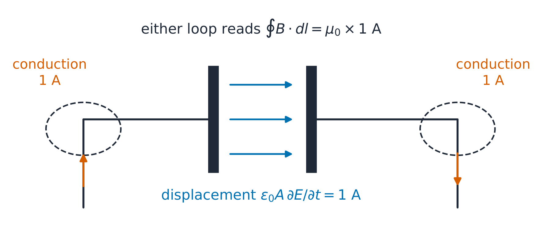
Start with the worked charging current of 1 A and compare a surface cutting the wire with one passing through the vacuum gap. The original law gives different predictions; including the changing-electric-flux term makes both totals equal. Change plate area to alter the field rate while its product with ε₀A remains the same current. Hold a nonzero stored charge to distinguish electric field from changing electric field.
Start with the worked 100 V/m RMS wave at 1 MHz. Its average power is about 26.5 W/m², while its instantaneous power at a field crest is twice that. Reinterpret the same number as a peak field and the average halves. Advance half a cycle to reverse E and H together without reversing the Poynting vector. Compare a uniform dielectric to vacuum, keeping the entered electric field specified.
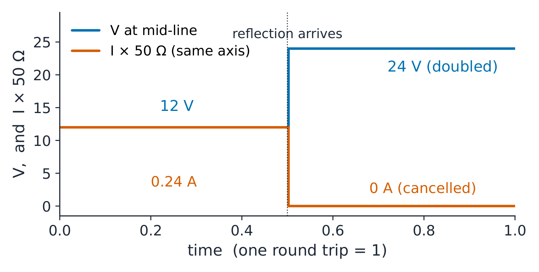
** worked example 2 — 開口端ステップ。** 50 Ω の transmission line を
12 V ステップで駆動し、開路とする。入射波は 12 V および
$12/50 = 0.24$ A。開放端では、$\Gamma = +1$:反射波+12 Vが倍化し
負荷電圧を24 Vとし、反射電流$-0.24$ Aが電流を打ち消す。
VSWR は無限大に近付くが、開路状態のシグネチャとして standing-wave メーターが読み取る値となる。
VSWRが無限大に近づくため、開放回路の特性は定在波の
計器の読み値となる。
一般的な誤り。$Z_{0}$を物理的な抵抗として扱う(それは
ratio; a lossless 50 Ω line dissipates nothing). Computing $\lambda$ with
$c$ instead of $v_{p}$ (30% error in PTFE). And forgetting the source-side
それを含める必要がある。
include it.
A 24 V source with 50 Ω series resistance launches the worked 12 V incident step. Follow its finite propagation delay to the open load, where voltage doubles and current cancels. Compare a short and a matched load, then change the source resistance to see whether the returning wave is absorbed or reflected again.
7.7
伝送管およびアンテナ
なぜ重要か。 ~10 GHz以上では同軸ケーブルの損失が大きすぎるため、ベンチリンクの
バックホール(およびすべてのレーダー)は中空パイプに移行し、
any radio link is always an antenna.
Common mistakes. Using the guide's NARROW dimension for $f_{c}$ (cutoff
is set by the wide one). Applying $\lambda_{g}$ as if it were $\lambda$ in Friis
(the free-space wavelength belongs there). And quoting dipole gain in dB
利得を dB だけで表記し、「i」を省略すること:2.15 dBi は等放射体に対する
相対値であり、ダイポールに対してはゼロとなる。
Start with WR-90 at 10 GHz and compare its 39.8 mm guide wavelength with the 30 mm free-space wavelength. Change the wide dimension and frequency to cross cutoff. The transverse field still fits the walls, but the axial pattern changes from a travelling wave to a decaying field. Near cutoff, its phase spacing becomes very long.