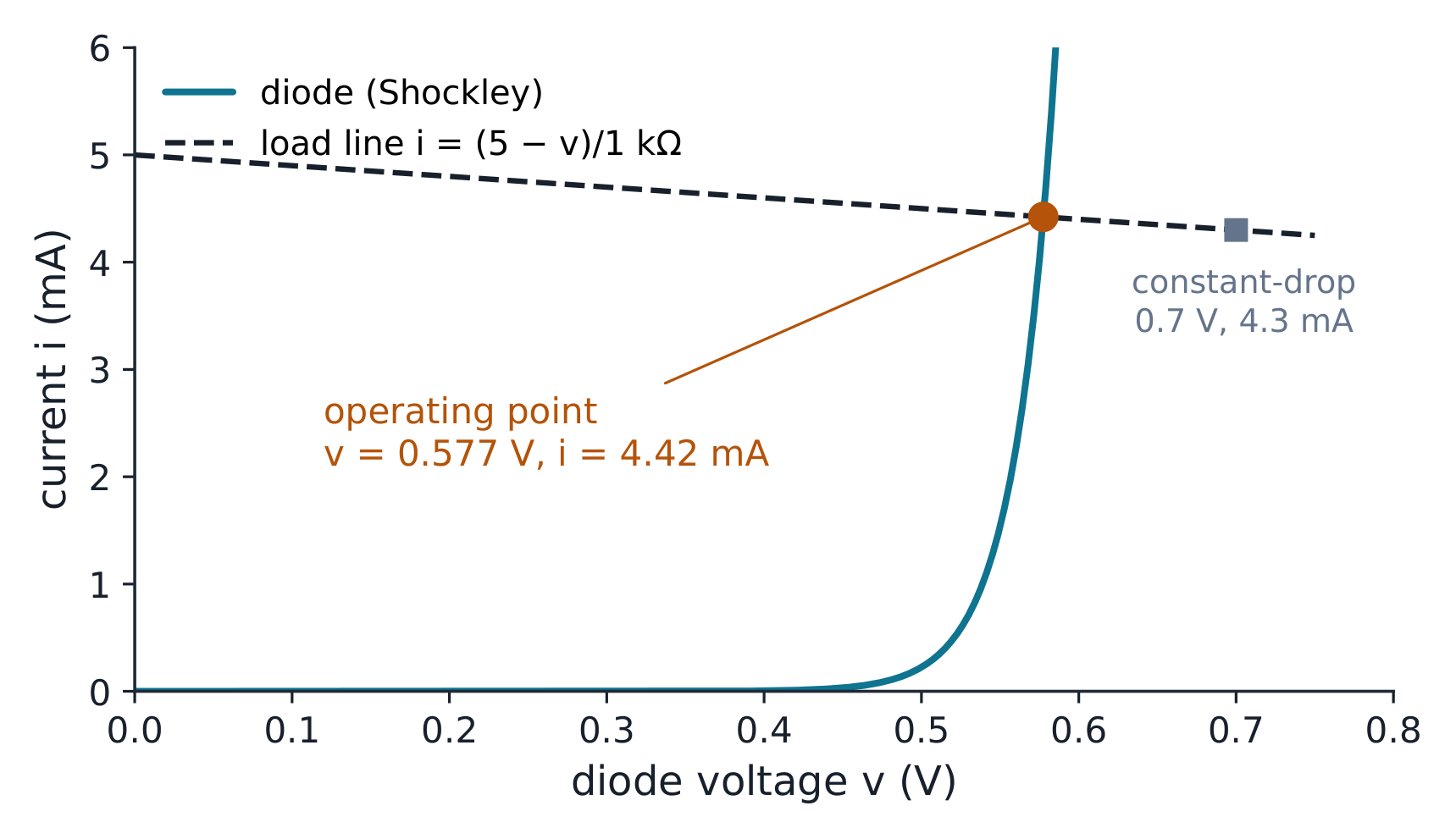
The 5 V and 1 kΩ circuit gives about 0.5775 V and 4.42 mA with Shockley, compared with 4.3 mA for the 0.7 V model. Change the source or resistor, then compare a +0.1 V source change with the local dynamic-resistance prediction. A low-supply case shows why a fixed drop can fail.
Full-wave bridge with 2200 µF at 100 mA: the capacitor bridges the gaps between peaks
** worked example 1 (ブリッジ電源、検証済み)。** ブリッジは 12 V の整流を行います
RMS、50 Hz二次側;負荷は100 mAを消費し、コンデンサは2200 µFである。
ピーク出力:$12\sqrt{2} - 1.4 = 17.0 - 1.4 = 15.6$ V。リップル(全波整流、
半周期ごとに10 msで再充電):$\Delta V = 0.1/(100 \times 2200\mu) = 0.455$ V。したがって
output lives between 15.6 and 15.1 V. Checks: ripple ≪ peak (2.9% ✓ — the
** worked example 0.91 (ツァーナーレギュレータ、両端で設計され、昇格済み)。
capacitor — the bridge buys a 2× for four diodes; PIV per diode ≈ 17.0 V (one
二次側ピーク) — その値より高いダイオードを選定してください。
Worked example 2 (a zener regulator designed at both extremes, escalated).
Regulate 12 V down to 5.1 V with a 5.1 V zener; the load varies
0–10 mA and the zener needs at least 2 mA to stay in breakdown. Worst case for
** worked example $R \le (12 - 5.1)/(10\mathrm{m} + 2\mathrm{m}) = 575\ \Omega$ (βが倍増、回路の要点、昇格済み)。同じ
560 Ω. Now check the other extreme — no load: $I_{Z} = (12 - 5.1)/560 =
12.3$ mA, so $P_{Z} = 5.1 \times 12.3\mathrm{m} = 63$ mW and the resistor
dissipates $(12-5.1)^{2}/560 = 85$ mW worst case. Full load leaves $I_{Z} =
12.3 - 10 = 2.3$ mA ≥ 2 mA ✓. Both extremes verified — that is a complete
レギュレータ設計です: 負荷範囲の両端からそれぞれ1つの不等式を用いています。
Common mistakes. Using f instead of 2f for the bridge ripple (the
capacitor recharges every half-cycle). Forgetting the 1.4 V of two diode drops
in the peak output. Sizing the zener resistor at the typical load only —
the zener current must be checked at BOTH extremes, and its power at the
無負荷極限。
For the 12 V to 5.1 V example, 560 Ω leaves 2.32 mA for the zener at a 10 mA load and about 63 mW at no load. With an illustrative 100 mW power rating, compare the lower power-bound resistance with the 575 Ω upper current bound. A smaller resistor can exceed the power rating; a larger one can lose regulation.
Worked example 2 (β doubled, the point of the circuit, escalated). Same
回路、$\beta = 200$: $I_B = 1.1/(10.2\mathrm{k} + 201\mathrm{k}) =
5.2\ \mu$A → $I_C = 1.04$ mA, $V_{CE} = 8.7$ V — まだ動作中 ✓。したがって β × 2
コレクタ電流を5%変化させ(0.99 → 1.04 mA)、Q点はほとんど
動かなかった。メカニズム:コレクタ電流の上昇はエミッタ電圧を
上昇し、これにより 減少$V_{BE}$ とベース電流を制限 — 負の
バイアス内のフィードバックは、$R_E$によって提供される。$R_E = 0$では、アクティブ領域の
公式$I_C = \beta(1.8 - 0.7)/10.2\mathrm{k}$はβ = 100で10.8 mAを予測する
β = 200で21.6 mAとなる。2.2 kΩのカスタマ电阻は、どちらの
12 Vからの電流も通過できないため、アクティブ仮定は成立しない:これらは候補である。
実際の飽和電流ではない。式におけるβの感度は依然として明確であるが、
Q点を受容する前に領域確認を行う必要がある。両方の誤差要因は現在定量化されている:分圧器由来の11%
ローディング(硬いデバイダで修正可能)、βのばらつきからの 5%(吸収されるため、
$R_E$).
Common mistakes. Checking $V_{CE} > 0$ instead of $> 0.2$ V (saturation
starts at about 0.2 V). Computing $V_C$ from the estimated 1.1 mA and then
"確認" exact currentから計算したQ点に対して — 一連の
チェーンを行って確認する。分岐器のみがバイアスをβに依存しないようにするとの誤解
のβ— 硬 enough のデバイダで $V_B$ を維持するために $R_E$ が
作業。
Keep the worked 12 V, 68 kΩ/12 kΩ divider, 2.2 kΩ collector resistor and 1 kΩ emitter resistor. Compare β = 100 and 200, then remove the emitter resistor or stiffen the divider. Check the active assumption before accepting any current or voltage as a Q-point.
よくある間違い。 領域の確認なしに飽和電流を信頼する
check (the failed example above sails through to a wrong answer if you only
$V_{DS} > 0$)。BJT(MOSFET の
飽和=増幅器;BJT 飽和=破滅)。ゲートの
電流は DC でゼロである— デバイダはローディングされていないが、それ故に
MOSFET デバイダはメガオーム抵抗可以使用する。
The worked 3 V gate gives a valid saturation point at 1.125 mA and 6.625 V. At a 5 V gate the saturation assumption fails, and the triode equation has two algebraic roots. Only 1 V and 3 mA satisfies the assumed region; the larger positive root is rejected.
** worked example 2 (ディージェネレーションとMOSFET比較、拡張版)。**
バイパスを外して$R_E = 1$ kΩを参加させる:正確な増幅倍は
$-g_m R_C/(1 + g_m R_E) = -84/(1 + 38.1) = -2.14$, against the $-R_C/R_E =
-2.2$ textbook form — within 2.4% because $g_m R_E = 38 \gg 1$(これがこの
形式の有効性条件であり、現在視覚的に確認できる)。ディージェネレーションは84を2.2に交換した——
直線性と安定した増幅倍が、バイアスを安定させた同一の$R_E$によって得られた。
bias. Same story in MOSFET land: the unit-5.4 Q-point gives $g_m = 2I_D/V_{ov} =
2 \times 1.125\mathrm{m}/1.5 = 1.5$ mS となり、コモンソース利得は
$-g_m R_D = -4.5$となる。同じ1.125 mAの条件下でBJTは$43.3$ mS —— 29倍の
MOSFETの——伝導度および電流増幅倍、無限大入力抵抗に対して:根本的なトレードオフ。
抵抗性を持つ:これが根本的なトレードオフである。
一般的な誤り。 正確な解が存在する後で、推定されたバイアス電流から$g_m$を計算すること。
小信号モデルが異なる回路であると信じる — 実際には同じ回路であり、Q点で微分したものである。
$-R_C/R_E$ where $g_m R_E \sim 1$ (the form needs $g_m R_E \gg 1$).
Believing the small-signal model is a different circuit — it is the same
circuit, differentiated at the Q-point.
Wave $g_m$'s金則が有限利得の視点と共に戻る。負のフィードバック
$r_\pi = \beta/g_m$; bypassed gain $-g_m R_C$, degenerated $-R_C/R_E$ when
開ループ利得$g_m R_E \gg 1$を用いて正確なノード方程式を書き、解くことで、
探索
A small-signal model is a tangent at the bias point
Start with the worked 0.99 mA BJT bias and recover gm about 38.1 mS, input resistance about 2.6 kΩ and bypassed gain about −80. Widen the input excursion to see the curved current law leave its tangent. Switch device at the same bias current to compare gm fairly, then select the MOSFET worked bias of 1.125 mA for gm 1.5 mS and gain −4.5.
導出(反転増幅段):オペアンプが1を維持できる場合、
closes a loop; what matters is the loop gain$A_{OL}\beta_{fb}$.
Derivation (inverting stage): if the op-amp can hold $v_- \approx v_+$, the
入力抵抗器には$(v_{in} - 0)/R_{in}$が流れ、フィードバック抵抗器にも
同じ電流が流れ、$v_o = -R_f v_{in}/R_{in}$となる。正確なノード方程式に
オープンループ利得$A_{OL}$を代入して解くと
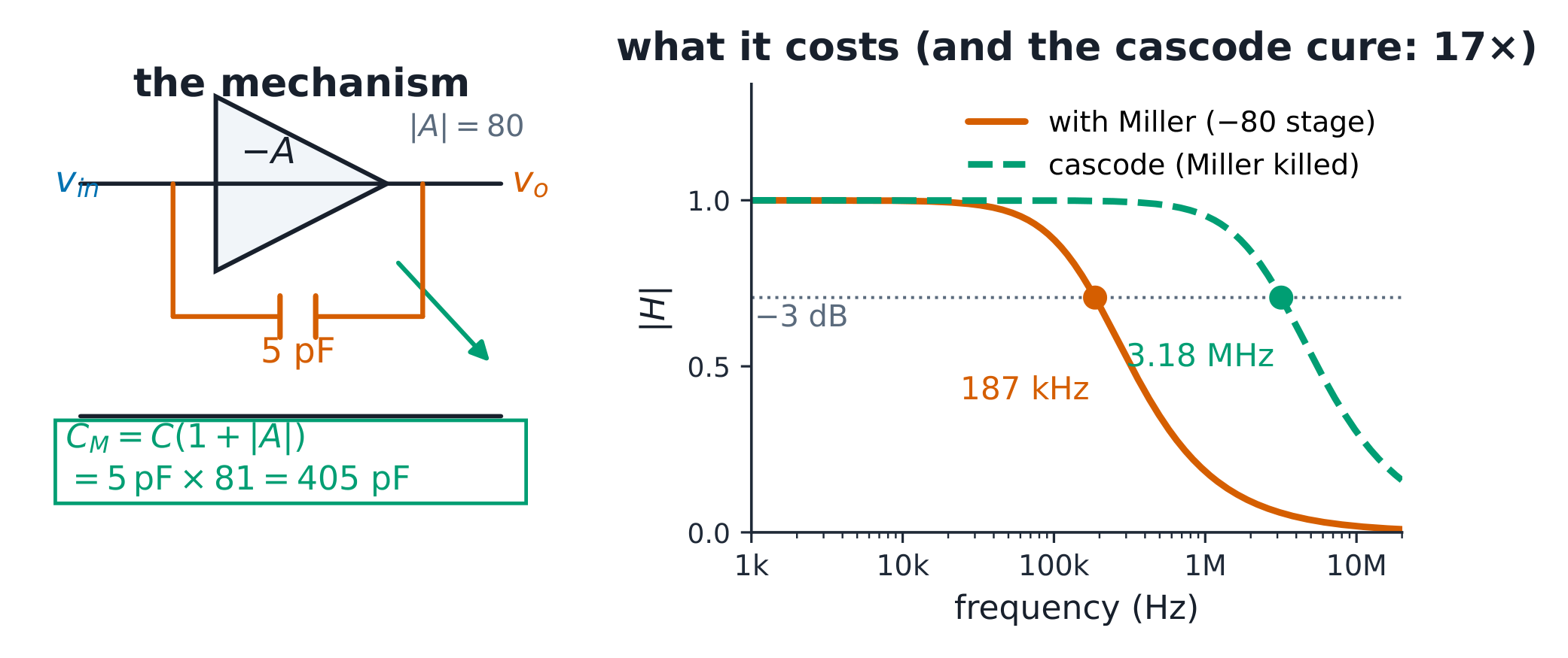
Miller moves the upper corner; cascades narrow both ends
$C_M=C(1+A),\quad f_H\approx\frac{1}{2\pi R C_{total}}$
Start with the worked gain magnitude 80, 5 pF feedback capacitor and 20 pF stray capacitance. Miller gives 425 pF in total and a high corner near 187 kHz. Suppress multiplication with the cascode idealisation to reach about 3.18 MHz. Then compare two buffered stages with one and probe the chain’s own half-power edge near 120 kHz. Changing the coupling capacitor moves the low corner independently.