電気工学のための数学的手法

これは大学電気工学の第2コースです：数学的 手法**——学位の残りの部分を支えるツールキットです。波 1 の直流回路 には代数のみが必要でしたが、交流回路以降、すべての手法はこのここで習う ものに依存しています。

• ユニット 2.1–2.3 は代数の復習と拡張を行います：信号のための微積分、複素数、 線形代数。
• ユニット 2.4–2.6 は動力学のツールキットです：微分方程式、ラプラス 変換、フーリエ級数。
• ユニット 2.7–2.8 は不確実性や場を取り扱います：ノイズのための確率論、電磁気学のためのベクトル 微積分。

各章は物語で始まり、形式的な概念の前に図を示し、用語を正確に定義し、後続の課程で引用される 結果を導出し、段階的に複雑になる二つの例題を解き、その数字は機械によって検証され、古典的な 間違いを列挙し、三行の要約で締めくくる。この習慣は学位全体で用いられる同一のものである: 具体的な値において すべての記号的答えを数値的に確認すること — 和による積分、代入による解かれた系、両辺を計算する変換対によって。 具体的な値において数値的に記号的な解答を得る—和による積分、解かれた 変数代入によるシステム、両辺を計算する変換対。

スコープトレースが0から5 Vまで滑らかに上昇して平坦になります。任意の瞬間におけるコンデンサへの電流は、トレースが移動する速さ、すなわち傾斜に依存します。 ある区間での電荷量は、電流トレース下の面積です。信号は時間の関数であり、微積分はそれらを読み解きます。 ある区間内で供給された電荷は、電流トレース下の面積である。信号は 時間の関数であり、微積分がそれらを読み取る：導関数 $dv/dt$とは 傾き—瞬間的な変化率；積分 $\int i\,dt$とは 蓄積された面積。

今後のEEの業務において、以下の3つの事実が大部分を担います：

• $e^{at}$ の導関数は $a\cdot e^{at}$ —— 指数関数の比率はそれ自身です 勾配。
• 矩形パルス（高さ$A$、幅$τ$）の積分は面積である。 $Aτ$.
• 三角形の面積は外接長方形の半分である—そして $\int_0^\infty A e^{-t/τ}\,dt = Aτ$ はその時間に対して指数関数的に減衰する $τ$の自己勾配の導出。 極限の定義：

Deriving $e^{at}$'s self-slope. The limit definition: $\frac{d}{dt}e^{at} = \lim_{h\to 0}\frac{e^{a(t+h)} - e^{at}}{h} = e^{at}\lim_{h\to 0\frac{e^{ah} - 1}{h} = e^{at}\cdot a$ — 指数関数的項は自身から外れる 差分商であり、これが$e^{at}$に比例して変化する回路が 微分においてその形を保つ理由である。

** worked example 1 （線形ランプ、検証済み）。コンデンサが 0 から 5 V まで 2 s で直線的に充電する（$v = 2.5t$）：$C = 100\ \mu F$ を用いると、$i = C\,dv/dt = 100\mu \times 2.5 = 250\ \mu A$ — ランプの傾きが一定であるため電流も一定である。送られた 電荷量は $\int i\,dt = 250\mu \times 2 = 500\ \mu C$ であり、これもまた $C \times \Delta V = 100\mu \times 5$. 2つの手法、1つの解答 — これが 確認の習慣です。

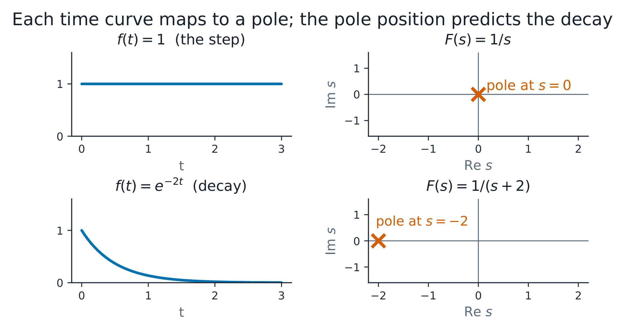
** worked example 2（指数パルス、拡張版）。** センサーパルスは $i(t) = 5 e^{-t/0.2}$ mA（ピーク5 mA、時間定数$τ = 0.2$ s）として減衰します。全電荷 面積 $\int_0^\infty 5e^{-t/0.2} dt = 5 \times 0.2 = 1.0$ mC に等しい — これは "有効幅則"が機能している例である。最大傾斜は $t = 0$ で: $\frac{di}{dt} = -\frac{5}{0.2} = -25$ mA/s. Check by crude summation: one rectangle of height 5 mA over the width 0.2 s gives exactly the same 1.0 mC — これは偶然ではなく $τ$ の意味そのものである。

**よくある間違い。**傾斜の値ではなくランプの値を微分すること （一定の5 V は一定電流を意味しない — 傾斜が一定时才意味する）。 積分が符号付きであることを忘れる：軸以下の面積は差し引く。 積分区内での単位を無視すること（$\mu A \times s = \mu C$、常に注意が必要）。

勾配を持ちます；パルスの面積は高さ×有効幅（減衰する 指数関数では$τ$）— かつすべての解答には単位があります。 指数関数など）— 答えには必ず単位がつく。

交流電圧は230 V および位相を持つ — 一つの数値では両方を表せないが、 平面上の点は可能である。複素数 $z = a + jb$（$j^{2} = -1$ を伴う）は実部、 虚部、絶対値 $|z| = \sqrt{a^{2} + b^{2}}$、および 変数 $θ = \text{atan2}(b, a)$。2つの形は互いに置き換え可能である：

— オイラーの恒等式は、電気工学（EE）で至る所で用いられる橋渡し的な関係です。積の演算は 位相を足し合わせます：$r_{1}e^{jθ_{1}} \cdot r_{2}e^{jθ_{2}} = r_{1}r_{2} e^{j(θ_{1}+θ_{2})}$ — 回転と拡大であり、これは正弦波の位相シフトや 振幅変化がどのように見えるかと同じです。

計算例 1（2つの位相ベクトルの除算、逆操作による検証） 除算を行う。 $6\angle 30^{\circ}$を$2\angle 80^{\circ}$で割る：極座標形式では答えは $3\angle -50^{\circ}$ そのまま — 絶対値は割り算され、位相は引き算されます。同じことを 直交座標形式で行う場合、$(5.196 + j3)/(0.347 + j1.970)$ の分母の有理化が必要です — 可能ですが、 極形式によるアプローチこそが、電気工学が フェーザー で機能する理由です。第3の確認方法： $3\angle -50^{\circ} \times 2\angle 80^{\circ} = 6\angle 30^{\circ}$ — 逆 演算は開始点に戻さなければなりません。

計算例 2（複素根を持つ二次方程式、拡張版） 減衰する の特性方程式 $s^{2} + 2s + 5 = 0$ の解は 行列式 $s = \frac{-2 \pm \sqrt{4 - 20}}{2} = -1 \pm j2$ は方程式が特異であることを意味し、一意な $2.236\angle \pm 116.6^{\circ}$ （絶対値 $\sqrt{1+4} = 2.236$）です。代入による確認： $(-1+j2)^{2} + 2(-1+j2) + 5 = (-3 - j4) + (-2 + j4) + 5 = 0$ が正確に成立します。解の 実部 $-1$が減衰定数であり、虚部 $2$ rad/s が振動の 一つの複素数が両方持ち備えているため、これがDegree（多項式の次数）の残りがそれらを一緒に保つ 理由となります。

** 一般的なミス。** 複素数の加算ではなく絶対値の加算を行うこと（絶対値は 加算を考慮せず、矩形成分のみを用いる。$e^{jθ}$の公式内では角度（度）を使用するが、これは ラジアンを前提としているため注意が必要。$j$の回転方向の混同：$j$倍すると$+90°$に なるが、$-j$倍すると$-90°$になる。

まとめ：2つの形、1つの数値 — 加算には矩形、乗除算には極形式。オイラーの恒等式がその架け橋であり、二次方程式の解は実部で減衰、虚部で振動数を表す。 および除算；オイラーの恒等式が橋渡しとなる；二次方程式の解は減衰を 実部に、周波数を虚部に持つ。

結合回路における3つのメッシュ電流は、3つの未知数に対する3つの連立方程式を意味し、 そして解の構造は「巧妙な置換」ではなく行列である。A 線形系 $Ax = b$は消去法で解かれ、行列の逆行列 $A^{-1}$が存在するのは行列式がゼロでない場合のみである。 2×2の場合：

行列式 $ad - bc = 0$ は方程式が特異であることを意味し、一意の解が存在しません。 解が存在せず、回路では依存源ループや浮遊ノードとなる。

2×2の逆行列の導出。 $A$にその候補を掛ける：$\begin{pmatrix} a & b \\ c & d \end{pmatrix} \frac{1}{ad-bc}\begin{pmatrix} d & -b \\ -c & a \end{pmatrix} = \frac{1}{ad-bc}\begin{pmatrix} ad-bc & 0 \\ 0 & ad-bc \end{pmatrix} = I$ — 交换と符号反転のパターンは、これらの 交差項が打ち消し合うからこそ存在する。

** worked example 1 （消去法と逆行列が一致）。$x + 2y = 8$、 $3x + y = 9$。消去法：行2から3×行1を引く → $-5y = -15$、したがって $y = 3$, $x = 2$. 逆行列式で検証：det $= 1\cdot1 - 2\cdot3 = -5$; $A^{-1} = \frac{1}{-5}\begin{pmatrix} 1 & -2 \\ -3 & 1 \end{pmatrix}$; $x = (1\cdot8 - 2\cdot9)/{-5} = 2$ ✓, $y = (-3\cdot8 + 1\cdot9)/{-5} = 3$ ✓。両方 経路が一致しており、それぞれが他方の検証となる。

** worked example 2 (メッシュ系、機械計算、昇格)。** EE01 2つのメッシュ回路は1つの行列方程式として整合する $\begin{pmatrix} 6 & -4 \\ -4 & 10 \end{pmatrix}\begin{pmatrix} i_A \\ i_B \end{pmatrix} = \begin{pmatrix} 12 \\ -3 \end{pmatrix}$。消元法（または 逆行列；det $= 60 - 16 = 44$）により $i_A = 2.455$ A, $i_B = 0.682$ A が得られ、 両元の方程式に代入して機械精度で検証済み。負の 非対角成分 $-4$ は共有抵抗器の表現である：結合は 非対角項として現れ、結合が強くなるほど行列式は 対角成分の積から遠ざかる。次に特異ケース：$x + 2y = 8$, $2x + 4y = 16$ の行列式は $1\cdot4 - 2\cdot2 = 0$ —— 第2式は just twice the first (a whole line of solutions, not one point).

** 一般的な誤り。** $A$ と $b$ の行順序を混同すること。 非ゼロ行列式は簡単な解を保証すると仮定すること——それは一意性を保証するのみで、 利便性を保証するわけではない。特異系には 解なし（平行な平面）や 無限大の解（従属する平面）があることを忘れること：行列式では どちらであるかを判別できない。 それである。

まとめ：行列式 ≠ 0 の $Ax = b$ は唯一の解を持ち、消去法でこれを求める。 逆変換で再導出され、代入により検証されます。結合は 非対角成分に存在します。det = 0 は幾何学的に崩壊したことを意味します。

スイッチが $t = 0$ で閉じると、コンデンサ電圧は新しい値へ滑らかに変化し— 波 1 の RC 応答は、この単元が一般化するパターンの一つの实例でした。この 回路方程式は常微分方程式です。一次の 定数係数を持つ線形ODEは、

解 = 斉次部分 $Ce^{-at}$ + 特解（強制項） により $f$。斉次項には初期条件が含まれる。

なぜ解がこのような形状になるか。 $\frac{dy}{dt} = -a(y - y_\infty)$ に対して、 $\frac{dy}{y - y_\infty} = -a\,dt$ に書き換えます：両辺はそれぞれ積分可能となり、 $\ln(y - y_\infty) = -at + C$ が得られ、すなわち $y - y_\infty = \tilde C e^{-at}$ です。最終値への乖離は 指数関数的に減衰します — すべての一次系は自身の百分率曲線に沿って滑り落ちます。 固有のパーセンテージ曲線。

** worked example 1 （ステップ毎に解いたRC回路、端点検証済み）。 $dy/dt + 2y = 10$、 $y(0) = 1$。斉次: $Ce^{-2t}$。特解（一定入力 → 一定値 $y_{p} = 10/2 = 5$ および $y = 5 + Ce^{-2t}$ となるため、方程式は $y(0) = 5 + C = 1$ と一致 ✓。これは $C = -4$: $y = 5 - 4e^{-2t}$。検証: $t = 0$ において、$y = 1$ ✓；$t \to \infty$ として、 $y \to 5$ and $dy/dt \to 0$, so the equation reads $0 + 2(5) = 10$ ✓. This is the 一般形における単位1.7のRC方程式 — このコースが教えるのは、回路そのものではなく、この手法です。 このコースで学ぶ内容である。

** worked example 2 （減衰する入力、機械検証済み、昇格版）。 解く $\frac{dy}{dt} + 3y = 6e^{-t}$、$y(0) = 2$。ある特解 $y_p = ke^{-t}$ を試す： $-ke^{-t} + 3ke^{-t} = 2ke^{-t} = 6e^{-t}$ gives $k = 3$. So $y = 3e^{-t} + Ce^{-3t}$; $y(0) = 3 + C = 2$ gives $C = -1$: $y = 3e^{-t} - e^{-3t}$. Check at $t = 0.5$: $y = 3(0.6065) - 0.2231 = 1.596$。左辺に代入すると： $dy/dt + 3y = -1.150 + 3(1.596) = 3.639$ となり、右辺は $6e^{-0.5} = 3.639$ — 機械精度と一致する。応答は2つの 指数関数に従い、入力の$(-1)$ とシステムの$(-3)$ である。

よくある間違い。 斉次方程式を解いてから、 particular part entirely. Letting the initial condition choose $k$ in the particular guess (only the homogeneous constant is free). Checking only $t = 0$: 大きな$t$ の極限についても確認する。このとき、式は整合する必要がある。 $dy/dt \approx 0$.

まとめ：同次解＋完全解；初期条件が家族から選択します。変数分離法は指数関数的な形状を説明します。両端でのチェックは任意です。 変数分離法は指数関数的な形状を説明し、両端のチェックを行う 両端は自由である。

Solving ODEs by hand works for one equation; a circuit with three storage elements needs three. The Laplace transform turns differentiation into multiplication by $s$, converting entire systems into algebra:

鍵ペアの導出. $\int_0^\infty e^{at}e^{-st}dt = \int_0^\infty e^{-(s-a)t}dt = \frac{1}{s-a}$ (for $\text{Re}\,s > a$) — the exponential eats its 単純な極を残す。この単一の計算が、表の大部分を生み出す。 表である。

有理$\mathcal{L}\{dy/dt\} = sY - y(0)$を逆変換可能な成分に分割する。 代数的に代入); $\mathcal{L}\{1\} = 1/s$; および部分分数 有理式$F(s)$を逆変換可能な成分に分解する。

** worked example 1 (単位2.4常微分方程式、変換による)。** $dy/dt + 2y = 10$を解く。 $y(0) = 1$. Transformed: $sY - 1 + 2Y = 10/s$, so $Y = (10/s + 1)/(s + 2) = 10/[s(s+2)] + 1/(s+2)$. Partial fractions: $10/[s(s+2)] = 5/s - 5/(s+2)$。したがって $Y = 5/s - 4/(s+2)$ であり、項ごとに反転させると：$y = 5 - 4e^{-2t}$ — 古典的な経路と同じであるが、 古典的な経路へ向かうが、初期条件は最終的な代数計算ではなく記録処理によって扱う。 $Y$の極（ここでは$s = 0, -2$）は、 振る舞いを予測する。

** worked example 2 (2次、機械検証済み、拡張版)。** $\frac{d^2y} {dt^2} + 3\frac{dy}{dt} + 2y = 0$, $y(0) = 1$, $y'(0) = 0$。変換: $(s^{2} + 3s + 2)Y = s + 3$ (the derivative rule applied twice), so $Y = \frac{s+3}{(s+1)(s+2)} = \frac{2}{s+1} - \frac{1}{s+2}$. Invert: $y = 2e^{-t} - e^{-2t}$. Checks: $y(0) = 2 - 1 = 1$ ✓; $y'(0) = -2 + 2 = 0$ ✓; $y(1) = 0.736 - 0.135 = 0.600$ (machine-verified). The two poles $-1, -2$ が 2つの減衰である。 遅い極$-1$が尾部を支配する — この観察結果は後に 課程で極支配近似となるという観察である。

よくある間違い。 微分規則における $-y(0)$ を忘れること（およびその 二階の対応する $-y'(0) - s\,y(0)$）。分数が完全に分解されていない $Y$ の逆数を取る: $\frac{s+3}{(s+1)(s+2)}$ は、それ以上の操作を行う前に2つの単純な部分に分割されなければなりません。 分子の零を極として読み取る（零はブロックし、極は減衰する）。 減衰する）。

要約: 微分 → $s$との乗算、初期値も含まれる; 部分 分数で$Y$を分解; 極は時間挙動を予測; 変換と 一致する——これが検証である。

歪んだ電源波形は、何らかの純正弦波の組み合わせによって抵抗器に同じように発熱する—— その組み合わせが推測ではなく計算であることを示す。任意の 周期信号は正弦波の和です。周期 $T$ に対して、基本 $ω_{0} = 2π/T$、フーリエ級数は

各 $a_{n}$ と $b_{n}$ は、対応する正弦波との内積である $f$ の平均値となります。 （直交性: 異なる正弦波は互いに平均してゼロになる—— したがって、各係数は独立して選べ、調谐フィルタのバンクのように）。 フィルタなど）。

** worked example 1 （四角波、魔法の点で検証済み）。** 四角 波 ±1、周期 $T$、奇対称性：すべての $a_{n} = 0$ および $b_{n} = 4/(nπ)$ が奇数の $n$ — 級数 $\frac{4}{\pi}(\sin\omega_0 t + \frac{1}{3}\sin 3\omega_0 t + \frac{1}{5}\sin 5\omega_0 t + \dots)$. The check that convinces: at $t = T/4$ において、 総和は 1 を与え、$\frac{4}{\pi}(1 - \frac{1}{3} + \frac{1}{5} - \dots)$ は $π/4$ のグレゴリー級数としてスケーリングされます — 1 に収束し、四角波が要求するように厳密に一致します。 すべての調和振幅は $1/n$ で減少します：鋭いエッジにはより多くの 調波が必要であり、これがフィルタリングの本質です。

** worked example 2 （調波内の電力、機械検証済み、拡大版）。** ±1 V 四角波が 1 Ω の抵抗に印加された場合、平均電力は 1 W です（一定 振幅の平均値）。パルヴァル定理により、調波の電力の総和も同じ 1 W となるべきです： $\sum_{n\ \text{odd}} \frac{1}{2}\big(\frac{4}{n\pi}\big)^{2} = \frac{8}{\pi^{2}} \big(1 + \frac{1}{9} + \frac{1}{25} + \dots\big)$. Summing the first 20 odd 奇数調和成分を合計すると0.990 W; 完全級数は厳密に1 Wに収束する（累加 逆奇数平方の和は$π^{2}/8$であり、これにより全体 要約：周期信号は調波に分解され、直交性によって各係数を独立して抽出する；エッジにおける振幅は $\frac{8}{\pi^{2}}\cdot\frac{\pi^{2}}{8} = 1$ で減少する；パルヴァルの定理は電力を検証する；ジブスの過渡は決して消失しない。 基本成分のみで電力の$\frac{8}{\pi^{2}} \approx 81\%$を担う — これは 第1調和成分のみを通過させるローパスフィルタでも、電力の大部分を供給する エネルギーであり、1/3-振幅の第3調和はわずか9%を加える。

よくある間違い。 基本振動数として$1/T$（ヘルツ）ではなく$ω_0 = 2π/T$（ラジアン毎秒）を用いること 各調和の電力における $\frac{1}{2}$ の無視（正弦波の平均二乗値は、最大値の二乗値の半分である）。 常に変対称であると仮定すること：原点をずらすと係数が変化し、スペクトルは配置された関数自体に属する。 原点と係数が変化し、スペクトルは関数全体に属するものとなる。 配置される。

要約：周期信号は調和成分に分解され、直交性によって各成分が 係数を独立して抽出します；端部における振幅は$1/n$に従って減少し、パルヴァルの定理は 電力を検証します；ギブズのオーバーシュートは決して消滅しない。

すべての測定にはノイズが含まれており、そのノイズ自体も予測不可能な信号であるが、 その 統計的性質 は安定しており、この安定性が計測器によって利用されている。 確率変数 は 確率分布 を持ち、 ガウス（正規）$N(\mu, \sigma^{2})$ が熱ノイズをモデル化する：

期待値 $E[X]$ は長期平均であり、分散 $Var(X) = E[X^{2}] - \mu^{2}$ はばらつきであり、$\sigma$ —— 標準偏差 —— はオシロスコープが表示するノイズの振幅である。 標準偏差** — オシロスコープが示すノイズ振幅である。2つの法則で 大部分の処理を行う：独立分散は加算される（$\sigma_{total} = \sqrt{\sigma_1^2 + \sigma_2^2}$), and the average of $n$ independent samples has standard deviation $\sigma/\sqrt{n}$.

**演習例 1（2σ則と平均化）。$X \sim N(0, \sigma^{2})$ $\sigma = 2$ mV において: $E[X] = 0$, $Var = 4$ (mV)², $\sigma = 2$ mV。確率は $\pm 2\sigma$ を超える確率は 4.55%（両尾の 95% 範囲は $\pm 1.96\sigma \approx \pm 3.9$ mV). Averaging 16 independent samples yields $2/\sqrt{16} = 0.5$ mV のノイズである——これが装置の平均化の全根拠である。

** worked example 2 （2つのノイズ源、dB計算、増幅）。アンプ stage adds 2 mV of noise to a signal that already carries 3 mV from the previous stage. The combined noise is not $3 + 2 = 5$ mV but $\sqrt{3^{2} + 2^{2}} = \sqrt{13} = 3.61$ mV ——分散は加算されるが偏差は加算されないため、 より小さいノイズ源は標称値よりも比例して寄与が小さい。 同じ 16 個の読み取りを平均した際の信号対雑音比の改善: $20\log_{10}(4) = 12.0$ dB。設計上の読取数：16回の測定で 12 dB 獲得され、さらに 6 dB ごとにコストがかかります。 4倍の測定回数（および4倍の測定時間）が必要となる；主要なノイズ源を 支配的なノイズ源をその発生源で除去すれば測定時間はゼロ — 3 mV を半分にすると 1.5 mV が $\sqrt{1.5^{2} + 2^{2}} = 2.5$ mV になり、各 3.2 dB の改善をもたらします。 単一測定ごとの改善効果である。

** 一般的な誤り。** 分散ではなく標準偏差を加算すること。 表や数式における $\sigma$ と $\sigma^{2}$ の混同（オシロスコープは σ を表示；数式 は通常 σ² を用いる）。$\sigma/\sqrt{n}$ の改善は 独立性を前提としていることを忘れる——相関ノイズ（商用電力ノイズ）は平均化によって除去されない。

まとめ：ガウス分布がノイズモデルであり、σ はオシロスコープのノイズであり、独立した 分散は加算され、平均化により σ は √n で割られます；支配的なノイズ源に攻撃し、その後 平均。

電圧プローブは空間の各点で一つの値を報告し、それにより一連の 値が形成される。この地形（景観）に関する記述がEE07におけるマクスウェル方程式である。 幾何学。場は位置のベクトル値関数である。位置に関する3つの演算子 場 $\mathbf{F}$:

• 勾配 $\nabla V$: スカラーの最も急な傾きの方向を指し、 電場は$E = -\nabla V$である。
• 発散 $\nabla \cdot \mathbf{F}$: 単位体積あたりの正味流出量—— 電場の電荷密度である。
• 回転（カール） $\nabla \times \mathbf{F}$: 単位面積あたりの循環量——静電気学ではゼロであり、 誘導現象のメカニズムとしてその場合のみ非ゼロとなる。

** worked example 1（勾配が低下を予測し、数値的に検証される）。** $V(x, y) = 3x^{2}y$ ボルト。$\nabla V = (6xy, 3x^{2})$；点 $(1, 2)$において： $\nabla V = (12, 3)$, so $E = -(12, 3)$ V/m. The check: move a small step $\delta = (0.01, 0)$ from $(1, 2)$ — $V$ changes by $\approx 6xy\cdot\delta x = 12 \times 0.01 = 0.12$ V, and $-E\cdot\delta = 12 \times 0.01 = 0.12$ V となる；これは 場とステップの積がポテンシャル低下を予測しており、これが勾配の意味である。

計算例 2（手による発散と回転、段階的拡大）。 $\mathbf{F} = (x^{2},\ xy,\ 3x^{2}z)$: $\nabla\cdot\mathbf{F} = 2x + x + 3x^{2}$, これは $(1,1,1)$ で $2 + 1 + 3 = 6$ に等しく — 正の発生源である。環流場について $\mathbf{G} = (-y,\ x,\ 0)$：回転の $z$ 成分は $\frac{\partial G_y}{\partial x} - \frac{\partial G_x}{\partial y} = 1 - (-1) = 2$ — 強さ 2の均一回転であり、剛体回転の速度場である。 body spinning at 1 rad/s, whose curl is twice its angular velocity. These two computations are the pointwise versions of EE07's ガウスの法則とストークスの法則。

一般的な間違い。 ベクトルの勾配やスカラーの発散を取る — 勾配はスカラー用、発散はベクトル用。回転の符号ミス： スカラーには勾配、ベクトルには発散を用いるという点の範例である。curlにおける符号ミス: $z$成分は $\partial F_y/\partial x - \partial F_x/\partial y$です; これらを逆転すると まとめ：勾配は最急勾配（スカラー→ベクトル）、発散は正味流出量

（ベクトル→スカラー）、回転は環流（ベクトル→ベクトル）；ステップは (ベクトル→スカラー)、カールは循環 (ベクトル→ベクトル)；ステップは整合性を図る必要がある $E \cdot \delta$ と $\delta V$ を整合させる。