制御システム

This is the tenth course in University Electrical Engineering: control systems. EE06 gave you the system function. This course closes a フィードバックループ 植物モデル（制御対象）の構築と、それを単一の伝達関数へ圧縮します。

• ユニット10.1と10.2は周波数領域で扱う：マージン、ナイキスト、PIDおよび 時間応答の予測と整形：仕様、安定性、ルーツロケーション。
• Units 10.3 to 10.5 predict and shape the time response: specifications, 状態空間への導入：多数の状態を持つモデルと、線形代数に基づく設計手法。
• Units 10.6 and 10.7 work in the frequency domain: margins, Nyquist, PID and 動的システムのモデル化
• Unit 10.8 opens state space: models for many states, and a design method built on linear algebra.

One habit runs through the whole course. Every design is checked in both domains. A phase margin predicts a damping. A pole placement predicts an overshoot. Every algebraic stability claim is confirmed by a second method: ルース法はルーツロカスに対して、ニュイ奎スト法はルース法に対して用いる。2つの異なるアプローチが同じ数値に到達したならば、その数値を信頼できる。 同一の数値に到達する道筋がある場合、その数値を信頼できる。

重要性。 クルーズコントロール搭載車が100 km/hで坂を走行する。3Dプリンター は、0.05 mmの範囲内でプラスチックの滴を配置する。両者は同じ方法で始まる：書き込み 物理系が何をするかを計算可能な方程式として記述する。

概念。 ほぼすべての物理領域は、エネルギーを蓄え、流れ、失う点で 共通のパターンを持つ。高温タンクは熱を蓄え、ヒーターから熱を得て、 部屋へ熱を失う。コンデンサは電荷を蓄え、電源から得て、抵抗器を通じて これらはそれぞれ「状態変数」$x$として表され、以下の式を示す。 各々は以下のように言う。

一次モデルは $\tau\, \dfrac{dx}{dt} + x = K\,u(t)$ の形を持つ。 The Greek letter $\tau$ (tau) is the time constant, measured in 秒である：蓄積が応答するのに要する時間を示す。記号$K$は DC gain: the final value of $x$ per unit of steady input $u$. With a step 入力$U$に対して、解は$x(t) = KU\,(1 - e^{-t/\tau})$となり、これが 最终値の63.2%に達するのは1つの時間定数の時点である。

線形化。実際の系は直線ではない。振り子 実在するシステムは直線ではない。振り子は$\ddot\theta = -(g/l)\sin\theta$に従うが、単一のゲインを持たない。対処法は、 から動作点（近傍で動作する状態）を選択し、置き換える 動作点（近傍で扱う状態）を選び、その地点における曲線の傾きによってそれを近似する。静止点付近では$\sin\theta \approx \theta$であるため、 振り子は固有振動数を持つばねのように振る $\omega_n = \sqrt{g/l}$。長さ$l = 0.9$ mのスイングに対して、$g = 9.81$ m/s²を用いて計算すると$\omega_n = \sqrt{9.81/0.9} = 3.30$ rad/sとなり、約0.53 Hzである：これは遅い 遊具のブランコ。同じ原理は、$q = 2\sqrt{h}$で排水するタンクにも適用される。 （m³/h で、$h$ は m）: 傾き $\dfrac{dq}{dh} = 1/\sqrt{h}$ は 0.5 に等しい。 $h = 4$ m 付近、および 1/3 が $h = 9$ m 付近にある。線形モデルは近傍でのみ有効である。 その動作点においてのみ成立し、傾きは正確さの度合いを示している。

** worked example 1: RC回路。** $R = 2$ kΩ と $C = 100$ µF を用いる。この 抵抗器には電流 $\dfrac{v_{in} - v}{R}$ が流れ、コンデンサには これを積分するため、

これは $\tau = RC = 2000 \times 100\times10^{-6} = 0.2$ s および $K = 1$ を持つ一次モデルである。入力信号を 0 から 5 V にステップ変化させると、コンデンサの電圧は $5(1 - e^{-1}) = 3.16$ V に達し、これは最終値の 63.2% であり、0.2 s で達成される。感度チェック：より大きな $R$ またはより大きな $C$ は回路の応答が遅くなることを意味し、積 ⟨$RC$⟩ の単位は seconds, so the model is consistent.

** worked example 2: アチュエータ制御DCモーター。** このモデルでは、 全体を通して選択する。モーターは転子慣性$J = 0.01$ kg·m²を持ち、 摩擦係数は $B = 0.1$ N·m·s、モーター定数は $K = 0.5$ (N·m/A 単位、数値上 V·s/rad と等しい) 、アチュエータ抵抗は $R = 1$ Ω である。インダクタンスは小さいため無視する。 無視できる。電気側と機械側を結びつける2つの物理法則が存在する： 以下の側面:

• トルクの法則: 電流がトルクを生み出し、$T = K\,i$、ここで $T$ は N·m 単位、$i$ は A 単位。
• ローターのニュートンの法則: $J\,\dot\omega = T - B\,\omega$、ここで $\omega$は軸回転速度（rad/s）である。

カップリングは双方向に動作します。回転するアーマチャラはまた、逆起電力（back-EMF） 電圧 $K\omega$ を発生するため、キルヒホフの電圧則 (KVL) は $V = R\,i + K\omega$ を与えます。初期条件がゼロの s 領域では、二つの法則は以下のようになります。

第2式を第1式に代入し、$\Omega$ の項をまとめます：

数値を代入します。分母は $0.01s + (0.1)(1) + 0.5^{2} = 0.01s + 0.35$ なので、

このモデルには极点が $s = -35$ rad/s にあります。時間定数は $1/35 = 28.6$ ms: 速い。DCゲインは最終速度の $50/35 = 1.43$ rad/s である。 DCでの感度確認：すべて一定の場合、モーター方程式は 純粋な代数であり、実際に $\dfrac{K}{BR + K^{2}} = \dfrac{0.5}{0.35} = 1.43$ となります。 過渡応答全体は3つの物理定数に由来し、逆起電力 は図において、モーターが自動的に形成するフィードバックループとして現れます。ここで 変数 $i$ と $\omega$ は、単位 10.8 が形式化する状態変数そのものです。

よくある間違い。

• KVLから逆起電力項 $K\omega$ を無視する。結果はより単純に見えますが、 は誤りである：$\dfrac{K}{(Js+B)R} = \dfrac{50}{s+10}$は5 rad/s per ボルトではなく1.43を予測し、時間定数が100 msではなく28.6 msとなる。この 逆起電力による内蔵フィードバックが、実際のモーターを高速にしている。
• 動作点から離れた線形近似を使用する。タンクの傾きは 0.5 $h = 4$ m および 0.33 $h = 9$ m で異なり、一つの傾きで両方を表すことはできません。
• 単位の混同：$J$ は kg·m²、$B$ は N·m·s、$\omega$ は rad/s です。 両方の法則でモーター定数が同じ値を持っているか確認してください。

要約. 蓄積、流れ、散逸が $\tau\dot x + x = Ku$ を与える。運転点を抉择し、傾きを取り代入すれば、その近傍で世界は線形になる。 運転点を抉择し、傾きを取り代入すれば、その近傍で世界は線形になる。 この Motor model $50/(s+35)$ はこれからの主要な例題となる。

重要性。 ブロック図とは、エンジニアがシステムを語るための表現である。 自動車のクルーズコントロールのポスターはブロック図であり、方程式のページではない。

概念. 伝達関数 $G(s)$ とは、初期条件ゼロでの s 領域における出力と入力の比である。ブロックが接続されれば、代数学ではなく演算が用いられる： 初期条件ゼロでの s 領域における出力と入力の比である。ブロックが接続されれば、代数学ではなく演算が用いられる： 接続されれば、代数学ではなく演算が用いられる：

• 直列（ブロックが連続する）：掛け算、$G = G_1 G_2$。
• 並列 (両ブロックが同じ加算点に入力): 和をとる、$G = G_1 + G_2$。
• フィードバック: ループで除算する、$T = \dfrac{G}{1 + GH}$。

フィードバック公式はその一行での導出に値がある。誤差は $e = r - H\,y$ であり、出力は $y = G\,e$ である。これらを組み合わせる: $y = G(r - Hy)$、移項して $GH\,y$ 項を移項して $y(1 + GH) = Gr$ を得る。この方程式

方程式は 特性方程式 である。その根は閉ループ極であり、安定性の全話を内包している。まず内部ループを縮小し、 その根は閉ループ極であり、安定性の全話を内包している。まず内部ループを縮小し、 すべての段階で分母を可視化しておくこと。

Worked example 1: one loop, read like a second-order system. Put $G_1 = \dfrac{1}{s+1}$と$G_2 = \dfrac{1}{s+2}$を$K = 6$のゲインで直列に接続する。 単位フィードバック（$H = 1$）下で：

次に、$s^{2} + 2\zeta\omega_n s + \omega_n^{2}$と照合して2次パラメータを読み取ります。ここで $\omega_n = \sqrt{8} = 2.83$ rad/s であり、 減衰定数 ⟨$\zeta = \dfrac{3}{2 \times 2.83} = 0.530$⟩ です。これは 標準設計領域 ⟨$0.4 \le \zeta \le 0.7$⟩ 内に位置し、単位が 10.3 これをおよそ 14% のオーバーシュートに変換します。

** worked example 2 ： 内包ループ。** 内部ループ ⟨$\dfrac{2}{s}$⟩ が フィードバックゲイン 0.5 は $\dfrac{1}{s+1}$ と直列に配置され、すべてが 単位フィードバックの外部ループ内にあります。ステップ ⟨1⟩ 、内部ループを圧縮する：

ステップ ⟨2⟩ 、直列ブロックを掛け合わせる：

ステップ ⟨3⟩ 、外部の単位ループを閉じる：

読み取る：$\omega_n = \sqrt{3} = 1.73$ rad/s と $\zeta = \dfrac{2}{2\times 1.73} = 0.577$ 。複雑な図が2つの数値に简化された。本当に複雑な 図に対しては、メイソンの増益法がこれを単一の式で行う：順方向パスの増益を合計し、接触しないループの積を差し引く。 ブロック代数が本当に複雑になった時にそれを目指すべきであり、それ以前には行わない；単純な図では ブロック代数が実際に複雑になる時、それ以前ではありません。単純な図では、 上記の3つのルールの方が速い。

よくある間違い。

• ループを $\dfrac{G}{1+G}$ で閉じる $H \ne 1$ の場合。帰還パスには $GH$ が含まれ、$G$ は含まれない。
• フィードバックサマのマイナス記号の喪失。誤差は $r - Hy$ である。もし 代わりに特性方程式は$1 - GH = 0$となり、すべての 安定性の主張が逆転する。
• 外側ループを最初に縮小する。動作はするが、代数的計算が爆発的に複雑になる; 内側ループを先に処理するのが作法である。

まとめ。 直列結合では掛け算、並列結合では足し算、フィードバック系では $1 + GH$ で割り算を行う。 結果の分母は特性方程式である。内側ループから順に処理する。 ループを先に処理する。

重要性。 ドローンメーカーが「半 秒以内に収束し、オーバーシュートが10%未満」と約束する場合、これらは時間領域の数値である。この単元 極点位置をこれらの数値に変換する辞書である。

概念。 2次系のプロトタイプには以下の用語が含まれる：

虚部は振動し、実部は $s = -\zeta\omega_n \pm j\,\omega_n\sqrt{1-\zeta^{2}}$ で減衰する。減衰比は極の角度のcosineであるため、原点から角度 $\omega_n$ のレイは一定減衰の線であり、一つの図、一つの数値となる。 虚部は振動し、実部 $-\zeta\omega_n$ は減衰する。減衰係数 は極点角度の余弦に等しいため、原点から角度 $\arccos\zeta$ の線は一定減衰の直線であり、一つの図、一つの数値となる。

ステップ応答とは、入力が 0 から 1 へ段階変化したときの出力である。 単位ステップ入力に対する標準的な結果は以下の通りである。

ここで $M_p$ はオーバーシュート（最終値以上のピークを 分数で表す）、$t_p$ はピーク時間、$t_s$ は設定時間 . オーバーシュート公式は魔法ではない：ステップ応答は

であり、最初のピークは導関数がゼロになる地点に現れ、それは $\omega_d t_p = \pi$；これを包絡式に代入すると $M_p$ となる。

定常誤差にはもう一つの概念が必要である。開ループ内の積分器の数を数える。その数が システムタイプ である。 開ループ側にある：この個数はシステムタイプである。タイプ-1 システム（一つ 積分器はステップ入力に対して定常誤差がゼロであり、その速度誤差 与える。速度誤差係数 $K_v = \lim_{s\to0}\, sG(s)$ はランプ誤差を $\dfrac{1}{K_v}$ で与える。計算前にループから定数を読み取る。 過渡応答である。

** worked example 1 ：二つの数値ペア、四つの仕様。** これを $\omega_n = 4$ rad/s および $\zeta = 0.5$。次に $\omega_d = 3.46$ rad/s および 極は $-2 \pm j3.46$ である。整合性の確認：原点からの距離は $\sqrt{2^{2} + 3.46^{2}} = 4 = \omega_n$ であり、当然如此である。仕様書：

10 から 90% までの 立ち上がり時間 は、ステップ応答から数値的に計算され、 応答を 0.41 s とする。異なる領域間での感度確認：$\zeta = 0.5$ は 位相余裕が約 50 度のときに来るべきであり、単位 10.6 の動作則 $\zeta \approx PM/100$ がループを閉じる。

** worked example 2: 減衰仕様を満たすためのゲインを選択する。** プラントは 単位フィードバックで $G = \dfrac{K}{s(s+2)}$ である。閉ループ系は $\dfrac{K}{s^{2} + 2s + K}$ であり、プロトタイプとの一致により $2\zeta\omega_n = 2$ および $\omega_n = \sqrt{K}$ が得られ、したがって $\zeta = 1/\sqrt{K}$ となる。要求： $\zeta = 0.45$:

応答を予測する：$M_p = e^{-\pi(0.45)/0.893} = 0.205$ であるため、20.5 %；ピーク 立ち上がり $t_p = \dfrac{\pi}{2.22 \times 0.893} = 1.58$ s; 定常化 $t_s \approx \dfrac{4}{0.45\times2.22} = 4.0$ s。ここで誤差定数を 開ループ: $K_v = \dfrac{4.94}{2} = 2.47$ と読み取ると、単位ランプに対して残る 誤差は $\dfrac{1}{K_v} = 0.405$ であり、ステップ誤差は正確にゼロである。なぜなら、 対象システムがタイプ 1 だからである。機械による検証: シミュレーションされた閉ループのステップ応答は 1.000 に定常化し、その最初のピークは 1.205 である。

よくある間違い。

• $\omega_n$ と $\omega_d$ の混合。ピーク時間は減衰振動数を用いる； 原点からの距離には $\omega_n$ を用いる。
• $t_s$ を帯域なしで引用する。2% および 5% の推定値は $\tfrac{4}{3}$ 倍の差がある。
• 極対が実際に優位であることを確認せずに、零点や追加の極を持つシステムに 二次系公式を適用すること。

要約。 極を入力として仕様を出力とする：$M_p$, $t_p$, $t_s$, および誤差 定数。極平面上の減衰線は一定過渡応答率線である。

重要性。 安定性は、他のすべての設計が成り立つ前に必須の特性である。自身を飽和状態に鳴らし続けるループは単に調整が粗いだけでなく、破綻しているのである。 他の設計上の問題がある。自身を飽和に導くループは tuning が悪いのではなく、 破損している。

** 概念。** クローズドループは、特性多項式のすべての根が負の実部を持つ場合にのみ安定である。 劳斯表（Routh array） 特性多項式は負の実部を持つ。 ラウス配列 は解くことなくそれらの根の個数を数える。係数を二つ 行を埋め、次に下方向に埋めていきます。各新しい値は、 その上の2つの行の積と商で求められ、第1列の符号の変化回数が 右半平面（RHP）の根の数に等しい。第1列に 符号の変化がない場合、RHPの根は存在せず：安定である。

計算例 1: RHPの根を数える。 $s^{4} + 2s^{3} + 3s^{2} + 4s + 5$ をテストする。

第1列は $1,\, 2,\, 1,\, -6,\, 5$ で読み取れる：2回の符号変化（$+1$ から $-6$ 、そして $-6$ から $+5$ へ）、したがってRHPの根が2つある。正確な根で確認すると、 $-1.29 \pm j0.86$ と $+0.29 \pm j1.42$ であり：実際に右半 平面に書き、配列は四次方程式を解かずにそれを示した。

計算例 2: ゲイン範囲を求める。 $s^{3} + 5s^{2} + 6s + K$ が安定となるための $K$ の条件は何か？ 配列を構築する：

安定には $\dfrac{30-K}{5} > 0$ と $K > 0$ が必要なので、$0 < K < 30$ 。 $K = 30$ にちょうど達したとき、$s^{1}$ 行が消滅する。これはエラーではない：完全なゼロ 行は対称根を示し、補助方程式から求めることができる。 その行の上にある行、$5s^{2} + 30 = 0$ 、から構築されるので、$s = \pm j2.45$ 。このシステム 境界上に位置する：臨界安定性、増大も減少もしない持続的な振動 2.45 rad/s で発生する。次の二単元はこの同じ ラウス検定は、どの根も解かれる前に安定な設計領域を描き出す

** 設計図。** ⟨$s^{3} + as^{2} + 8s + K$⟩ の族に対して、同じ 外積は $s^{1}$ 成分 $\dfrac{8a - K}{a}$ を与えるため、安定性は ちょうど $0 < K < 8a$ ： $(a, K)$ 平面上の直線境界である。このコースの実行 植物 $s(s+2)(s+4)$ は、$a = 6$ と限界 $K = 48$ を持ち、後続のすべての単位がその同一の点に収束する。 後の単元がこの同じ点に到達する。

よくある間違い。

• 不完全な多項式を配列に入力する。係数は $s^n$ から下位のすべてのべき乗をカバーする必要があり、欠落したべき乗には係数 0 が割り当てられる。
• 簡略化のため、行を負の数で割る。正の数による再スケールは自由であるが、負の再スケールは計算対象の符号自体を反転させる。 数は自由である；負の再スケーリングは、あなたが数えている符号そのものを反転させる。
• Treating a single zero in the first column as failure. Replace it with a small positive $\varepsilon$ and continue; a whole zero row needs the 補助方程式が必要である。
• $K = 30$ ケースを「安定」と呼ぶ。軸上の極は安定ではなく、限界安定であり、振動は決して消滅しない。 ターニングセッションが行われる。ルーツローカスは、閉ループ極がどこへ向かうかを示している。

まとめ。 配列を構築し、第一列の符号変化数を数えれば、ルーツファインディングを行うことなく右半平面の根数が得られる。パラメータ範囲は1つの行から読み取れる。 何ら構築する前でも、それを回すことでわかる。

重要性。 ゲインは、増幅器、コントローラー、チューニングセッションのすべてで操作されるノブである。ルート locus は、何ら構築する前に、これが回転されたときに閉ループ極がどこへ向かうかを示す。 調整セッションが行われる。ルーツロケーションは閉ループ極点がどこへ移動するかを示す 極と零点の和がその右側にある。

概念。 ルーツロケーションは、$s$において ループ $L(s) = K\,\dfrac{\prod(s-z_i)}{\prod (s-p_i)}$ に対して角度条件が成立する:

各枝は開ループ極点 ($K = 0$ に位置) から始まり、零点または 無限大に終わる。標準的な概略図の描画ルールはすべてこの1つの条件から導かれる:

• 実軸上の区間: 右側に極点と零点の合計数が奇数個ある場合のみ、その区間にルーツロケーションが存在する。 ポールとゼロの和がその右側にある点の集合である。
• 漸近線の角度$\dfrac{180°(2k+1)}{n-m}$、重心に中心を置く 実部と虚部の両方を解く。
• 分岐点（枝が実軸から離れる点）は、 $\dfrac{d}{ds}\Bigl[\dfrac{\prod(s-p_i)}{\prod(s-z_i)}\Bigr] = 0$であり、ルーツロケーション上の根のみが有効である。 roots on the locus count.
• The $j\omega$-axis crossing: put $s = j\omega$ into $1 + KL_0 = 0$ and solve the real and imaginary parts.

Worked example 1: sketch the running plant. Take $L = \dfrac{K}{s(s+2)(s+4)}$. Three poles at $0, -2, -4$ and no zeros, so $n - m = 3$ and the asymptotes leave the centroid $\dfrac{(0) + (-2) + (-4)}{3} = -2$ at $\pm 60°$ and $180°$. The real-axis locus is the segment $[-2, 0]$ and the half-line $(-\infty, -4]$. The breakaway solves

giving $s = -0.845$ (on the locus: keep it) and $s = -3.155$ (between $-4$ および $-2$、軌跡外にある場合: 除外する）。離脱点におけるゲインは $K = |s(s+2)(s+4)| = 0.845 \times 1.155 \times 3.155 = 3.08$ である。$j\omega$ 交差点: $s = j\omega$ との交点において、実部は $K = 6\omega^{2}$ を与え、虚部は imaginary part gives $\omega^{2} = 8$, so $\omega = 2.83$ rad/s and $K = 48$. Routh境界が示した同じ 48 である。

極が移動し、−0.845で合流し、漸近線に曲がり、K = 48で不安定領域へ進入する「

** worked example 2: 軌跡上の減衰仕様設計。** 要求条件は $\zeta = 0.5$である。極は負の実軸から$\arccos 0.5 = 60°$の角度を持つ放射線上に位置し、すなわち negative real axis, that is on $s = -\sigma + j\,\sqrt{3}\,\sigma$ for some $\sigma > 0$. Search along the ray for the point that satisfies the angle condition. At $\sigma = 0.667$ the three pole angles are $120° + 40.9° + 19.1° = 180°$ exactly, so the design point is

gain（ゲイン）は大きさ条件より得られる：

幾何学的確認：$|s^{*}| = \sqrt{0.667^{2} + 1.155^{2}} = 1.334$および $\dfrac{0.667}{1.334} = 0.500$ となり、要求された減衰に完全に一致する。安定性マージンの 確認: $K = 8.30$ は限界 48 よりも十分に下位に位置するため、減衰は $\zeta$に位置し、対を左側に大きく離しているため、対が支配的となり $-4.67$ ではなく、対の左側に十分遠くにあるため、この対が支配的となり 2次近似が成立する。

よくある間違い。

• Keeping an off-locus breakaway root. The quadratic gives two answers; only 軌跡上の点のみが物理的に意味を持つ。
• Reading damping as distance from the origin. $\zeta$ is the cosine of the pole angle: circles are constant $\omega_n$, rays are constant $\zeta$.
• Assuming the asymptote crossing is the $j\omega$ crossing. Compute the $1 + KL_0 = 0$ からの交点；漸近線は概略図の補助に過ぎない。

要約。 角度条件を考慮して、線分、重心、漸近線を概略描画する。 離脱点、交差点。設計とは、減衰線に位置を移動させて 利得を読み取ることである。

重要である理由。 実務では極の正確な位置はほとんど未知であり、 周波数応答を測定する。マージンとは、その測定値に基づいて示される工学的許容差であり、このループが不安定にどれだけ近いかを示す指標（デシベルと 度で）である。 度（°）か？

概念。 ボード線図はループ利得 $L(j\omega)$ を、振幅（単位 dB（対数周波数に対して）および位相（度）。各極は、 $-20$ dB/decade の傾きと最大 $-90°$ の位相寄与を持ち、各零点は その逆の寄与をする。プロットから読み取れる2つの値が安定性情報を示す：

• 位相余裕 PM：ゲイン・クロスカッス周波数 （$|L| = 1$ となる点）において、位相が $-180°$ より上にある度数。
• ゲイン余裕 GM：位相・クロスカッス（ $\angle L = -180°$ となる点）において、$|L|$ が 1 より下にある倍率。

領域同士を結びつける実務則は $\zeta \approx PM/100$ である： 50° の位相余裕は $\zeta \approx 0.5$ に相当し、オーバーシュートは 16% 前後となる。 ニュイキストの判定法は安定性のカウントを正確にする。プロット $L(j\omega)$ が $\omega$ から $-\infty$ へ $+\infty$ となる際、時計回りに 巻回数 $N$ を $-1$ の点の周りに取り囲むと、閉ループ系には $Z = N + P$ の右半平面極が存在する。ここで $P$ は開ループ系のRHP極数を表す。（原点にある 極は、当例の植物のようにニュイキスト 曲線において右側に_indentation_される；その無限弧は $-1$ から遠く離れており、ここでは影響しない。）

このときの位相は 1 であり、したがって $L = \dfrac{100}{s(s+10)}$ 。ゲイン・クロスカッスは $|L| = 1$ を解くことで求められ、つまり $\omega\sqrt{\omega^{2}+100} = 100$ である。両辺を二乗すると $\omega^{4} + 100\omega^{2} - 10^{4} = 0$ となるので、

このときの位相は $-90° - \arctan(7.86/10) = -90° - 38.2° = -128.2°$ であり、したがって 位相余裕は $PM = 180° - 128.2° = 51.8°$ となる。ゲイン余裕は無限大： 位相が $-180°$ に漸近的に近づくのみである。時間領域で検証する。 領域において、閉ループ系は $\dfrac{100}{s^{2} + 10s + 100}$ であり、まさに ルール$\omega_n = 10$は、正確な16.3に対して$\zeta = 0.5$を予測した：これは有効な推定値であり、定理ではない。 実則 $\zeta \approx PM/100$ は、厳密な 0.5 に対して 0.52 を予測した：実用的な 推定値であり、定理ではない。

Worked example 2: the running plant, three ways. Take $L = \dfrac{20}{s(s+2)(s+4)}$, the $\zeta = 0.5$ design with the gain more than doubled. The phase reaches $-180°$ where the imaginary part of $s(s+2)(s+4)$ vanishes, at $\omega = \sqrt{8} = 2.83$ rad/s, and there

The gain crossover solves $\omega\sqrt{\omega^{2}+4}\sqrt{\omega^{2}+16} = 20$, giving $\omega_{c} = 1.73$ rad/s. The phase there is $-154.3°$, so $PM = 25.7°$. The rule predicts $\zeta \approx 0.26$ and a ringing response; 完全な閉ループをシミュレートすると48%のオーバーシュートが得られ、これが マージンが保証する挙動である。次にニュ奎ストチェックを行う。$-180°$における 周波数での増幅は$K/48$であり、したがって$K = 20$において曲線は0.42の right of $-1$: no encirclement, stable. At $K = 48$ it passes exactly through $-1$: marginal. At $K = 96$ it wraps twice clockwise around $-1$, so $Z = N + P = 2 + 0 = 2$ closed-loop RHP poles. Routh on $s^{3} + 6s^{2} + 8s + K$ $K > 48$に対して不安定であると示し、右半平面に2つの根を持つ $K = 96$。3つの手法、 1つの答え。

よくある間違い。

• 閉ループ応答からマージンを読み取る。マージンはループ内に存在する gain $L$、ループが閉じる前。
• 2つのクロスオーバーを混同する。PMはゲインクロスオーバーに対応し、GMは フェーズクロスオーバーに対応する。
• 原点の周回数を数える。基準は交差の 点 $-1$、この符号の定義では反時計回りが正である 方向。
• $P$を忘れること。植物自体に右半平面極がある場合、$Z = N + P$がその カウントが必要であり、$N$だけでは答えにならない。

まとめ。 ボード線図はPMとGMを秒単位で示し、$\zeta \approx PM/100$が それらを時間領域に変換する；ニュキスト線図は右半平面極を正確にカウントし、これら3つはすべてラウス判定と一致する必要がある。 Routhと一致しなければならない。

なぜ重要か。 多くの産業ループはPIDを動作させています。これはあなたが最初に調整し、最も頻繁に調整することになるコントローラーです。 あなたが調整すべきコントローラであり、最も頻繁に調整することになるコントローラである。

考え方。 PIDコントローラはPIDが誤差 $e = r - y$に対して 同時に3つの方法で作用する：

比例項は現在に応答します。積分項は記憶に残ります：システムタイプを上げることで定常誤差を除去します。 記憶する：システムタイプを上げることで定常誤差を除去する。また、 微分項は予測を行い、速さに比例する減衰を加える。 $u = K_{p}\bigl(e + \frac{1}{T_i}\int e\,dt + T_d\dot e\bigr)$ 積分時間 $T_i$ と微分時間 $T_d$ は、どちらも秒単位である。

古典的な最初の試みはジグラー・ニコルズの限界ゲイン調整である：ループがわずかに振動するまで比例ゲインを上げ、 限界ゲイン $K_u$ と振動周期 $T_u$ を記録し、表の該当行を参照する。価格表はゲインと同じくらい重要である。Pだけでは定常誤差を完全に消除できない。Iは位相遅れを追加する。Dは測定ノイズを増幅するため、参照値ではなく測定出力に対して作用させなければならない。否则、すべての設定値変更 価格表もゲインと同様に重要である。Pのみでは定常誤差を 完全に除去できない。Iは位相遅れを加える。Dは測定ノイズを増幅し、 設定値の変化ごとに、 作動器を駆動する。

** worked example 1: 動作中の株に対するジーグラー-ニコルズ法。** ループ $\dfrac{K}{s(s+2)(s+4)}$は$K_u = 48$で$\omega_u = \sqrt{8} = 2.83$ rad/s（ラウスとニュイストの境界）で振動するため、周期は$T_u = \dfrac{2\pi}{2.83} = 2.22$ sである。表のPID行から以下の値が得られる。

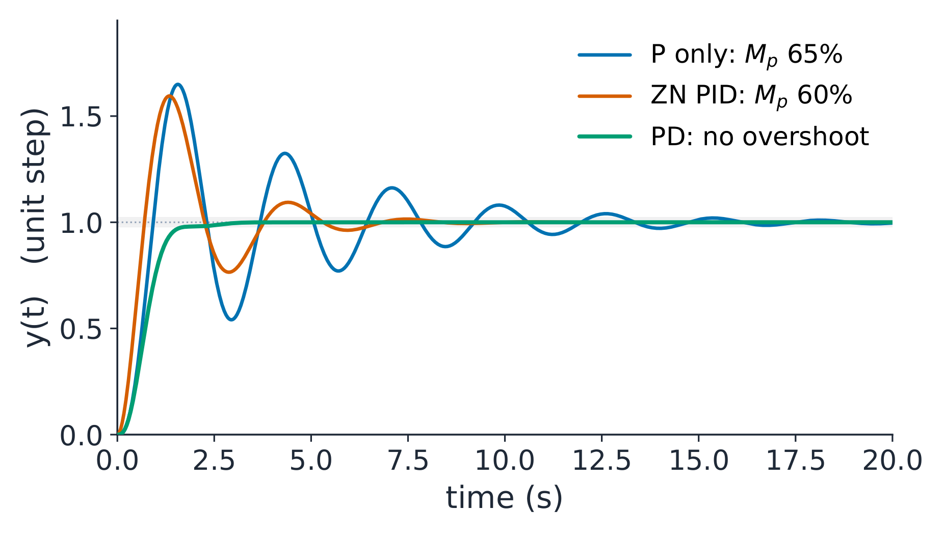
実際に何を得るか？Pのみを$K_p = 28.8$に設定した場合、閉ループ $s^{3}+6s^{2}+8s+28.8$には極点$-5.50$と$-0.25 \pm j2.27$があり、過渡応答は65% オーバーシュート、15 sでの<(), 定常ランプ誤差 $\dfrac{1}{K_v} = \dfrac{8}{K_p} = 0.278$。Ziegler-Nichols PIDはこの誤差を除去する 完全に取り除き、積分器がタイプを上げるためであり、最初のオーバーシュート is 60%, decaying to about a sixth each cycle: the recipe aims at a quarter-decay, not at comfort. The honest lesson: the table lands 一度の実験で近傍に到達させるが、作業を完了させない。

計算例 2：微分項で終了し、リードサイズを決定する。 $K_p = 28.8$を維持して微分項を追加する。PDループの特性多項式は $s^{3} + 6s^{2} + (8 + K_{p}T_d)s + K_{p}$である：D項は文字通り減衰係数に追加される。 damping coefficient. Raise $T_d$ from the Ziegler-Nichols value until the 極点は$T_d = 0.5$と$s^{3}+6s^{2}+22.4s+28.8$である。微分項が作用する位置が重要である： with poles $-2$ and $-2 \pm j3.22$. Where derivative acts matters: on the measurement (the right practice, as below) the reference step meets no 誤差に対して、2.1におけるPD零点は実極点を相殺し、残る On the error the PD zero at $-2$ cancels the real pole and the surviving pair, $\zeta = 2/3.79 = 0.53$, still rings at about 14%: damping either way, but only the measurement form is kick-free. The ramp error stays $0.278$: derivative buys damping, not accuracy. For accuracy and speed together you 項を統合して再調整し、これが10.7の exercises に完全に相当する。

極を持ち、ある周波数で位相を増加させる。最大増加量は 補償は同じ役割を果たす。リード补偿器 $\dfrac{1+\tau s}{1+\alpha\tau s}$ と $0 < \alpha < 1$ は、位相をある周波数で買収するゼロを極より下に配置する。最大位相上昇量は ある周波数において位相と位相_sharedを购买する。最大リフトは

For a +45° lift, $\alpha = \dfrac{1-\sin 45°}{1+\sin 45°} = 0.172$. The same network also lifts the high-frequency gain by $\dfrac{1}{\alpha} = 5.8$, 設計がこれを受け入れなければならない場合、通常は主利得を下げることによって行われる。遅れ ネットワークとは、$\alpha > 1$を持つ同一のペアであり、低周波帯域での利得を得るために利用される。 アンチ・ウィンドアップ は、実際の実装に必ず含まれるべき要素である。アクチュエータが飽和すると、

積分器は消費できない誤差の蓄積を続けるため、回復時には蓄積された作用を一つの大きなオーバーシュートとして放出する。二つの 標準的な対処法は、出力が飽和している間は積分器をクランプするか、 逆計算を行い、飽和 excess（過剰分）にゲインを掛けてフィードバックして積分項を減少させるかである。これらのいずれかがない場合、最初の実際の飽和は設計したすべての マージンを食い潰してしまう。 逆算して、飽和過剰分に利得を掛けてフィードバックし、 代わりに表のステップ応答変種を使用すべきである。 設計したマージンを回復させる。

よくある間違い。

• 振動しない植物に対して最終利得法を実行すること。この 一次系または重度減衰植物には$K_u$が存在しないため、ステップ応答 表の代替バリアントを使用する。
• 測定値ではなく誤差の微分を行うこと。セットポイントステップ は無限の傾きを持ち、D項がアクチュエータを駆動する。
• 調整形式を混同する。系列定数 $K_p, T_i, T_d$ は 並列ゲインではない：$K_i = K_p/T_i$ と $K_d = K_p T_d$ 。
• リードネットワークを設計して、その $\dfrac{1}{\alpha}$ を忘れる 高周波ゲインの引き上げは、購入したマージンを削ぐことにつながる。

まとめ。 Pは反応し、Iは記憶し、Dは予測します；それぞれが一つの振る舞いを買って、 既知の価格を支払います。最初のカットには表を使い、マージンで 微調整を行い、アンチ・ウィンドアップで現実味を持たせます。コース ページのインタラクティブラボでは、これら二つのノブであるゲインと減衰を正確に操作でき、 オーバーシュート、settling time、安定性がどのように動くかを確認できます。

なぜ重要か。 伝達関数は一つの入力と一つの出力を記述します。 現代のコントローラーは、バランスロボットや四つのループを同時に動作させるドローンなど、 複数の内部変数がモデル化され、統合されてフィードバックされるステートスペース上に存在します。 フィードバックされる。

$n$ 個の一次方程式としてシステムを表します： 単一の$n$次多項式ではなく、以下の連立方程式を用いる：

ここで、$x$は状態ベクトル、$u$は入力、$y$は計測出力である。 $A$, $B$, $C$, $D$ は定数行列である。直感的な解釈：状態は$n$の drawers of memory. The matrix $A$ says how each drawer pushes the others, $B$は入力がどこから入るかを示し、$C$は何を測定するかを示す。 $A$の固有値はシステムの極です。なぜなら、 $\det(sI - A) = 0$ はちょうど特徴方程式だからです。零入力では、解は $x(t) = \Phi(t)\,x(0)$であり、ここで遷移行列 $\Phi(t) = e^{At}$は無限級数として計算される行列指数関数です。 級数 $I + At + \dfrac{(At)^{2}}{2!} + \cdots$であり、すべての 正方行列に対して収束します。

** worked example 1: モデルを読み取り、その減衰を確認する。** $G(s) = \dfrac{8}{(s+2)(s+4)} = \dfrac{8}{s^{2}+6s+8}$とする。コンパニオン形では、

DCゲインは構成を検証する：$-CA^{-1}B = \tfrac{8}{8} = 1$, $s = 0$におけるプラントゲインと一致する。$A$の固有値は$-2$および $-4$であり、ちょうど極である。次に、遷移行列を$t = 0.5$ sで評価し、 級数によって計算する：

その固有値は$e^{-1} = 0.368$と$e^{-2} = 0.135$である：各極は半秒あたり自身の減衰係数となる。これが深い同一性である：行列 半秒ごとに独自の減衰因子を持つ。これが本質的な同型性である：行列 指数関数は極であり、実数化されたものである。$x(0) = [1,\;0]^{T}$から始めると、 すべての軌道が遅い固有ベクトル0.5に直線化されるため、$[0.600,\; -0.930]^{T}$極が応答の尾部を支配している。 位相平面においてすべての軌道が緩やかな固有ベクトル$[1, -2]^{T}$に沿って直線化され、そのため$\lambda = -2$極が 応答。

Worked example 2: pole placement by linear algebra. With full-state フィードバック $u = -K_{fb}\,x$（ここで $K_{fb}$ はゲインの行ベクトルであり、ループゲインではない） loop gain), the closed-loop matrix is $A - BK_{fb}$ and you choose its その特性多項式は $-10$ となります。一致させます。 $s^{2} + 20s + 100$. With $B = [0,\;1]^{T}$ and $K_{fb} = [k_1,\; k_2]$,

whose characteristic polynomial is $s^{2} + (6+k_2)s + (8+k_1)$. Match 性質は 可制御性 であり、行列 $k_1 = 92$ のランクによって確認され、ここでは $k_2 = 14$ であるため、両極を配置可能である。 eigenvalues of $A - BK_{fb}$ compute to $-10$ and $-10$ exactly. What the 根軌道法が光線の沿って探索することで達成したことを、状態フィードバックは連立一次方程式を解くことで達成している。 直列補償器の組み合わせでは到達できない極を配置できる。ただし、入力が実際にすべての状態方向を駆動できる場合に限りである。 reaches, provided the input can actually drive every state direction. That property is controllability, checked by the rank of the matrix $[\,B\;\;AB\;\;\cdots\,]$, which is 2 here, so both poles are placeable. When the states are not measured, an observer estimates them; that is the door to the next course.

よくある間違い。

• Forgetting $C$. The states are not the output; the transfer function is $C(sI-A)^{-1}B + D$, and dropping $C$ quietly changes the DC gain.
• Taking $e^{At}$ element by element. The matrix exponential is defined by このシリーズ、およびその非対角成分は指数関数ではない 成分である。
• ポール配置が常に機能すると仮定する。$[\,B\;\;AB\;\;\cdots\,]$が失われると、 ランク、一部の方向は到達不可であり、$K_{fb}$が存在しません；確認 可制御性をまず確認してください。
• 混合の慣例。このコースでは列状態と行$K_{fb}$を使用します； 行状態を用いる教科書ではすべての積が反転されます。

要約。 $A$はダイナミクスを保持し、その固有値は極であり、$e^{At}$ は自由応答であり、$u = -K_{fb}x$は設計を線形代数に変換し、 可制御性によって保証されます。