The normal distribution · La loi normale
| English | Français |
|---|---|
| normal distribution/ˈnɔːml ˌdɪstrɪˈbjuːʃn/ | distribution normale |
| continuous variable/kənˈtɪnjuːəs ˈveərɪəbl/ | variable continue |
| standardize/ˈstændədaɪz/ | standardiser |
| approximate/əˈprɒksɪmət/ | approximer |
| continuity correction/kɒntɪˈnjuːɪti kəˈrekʃn/ | correction de continuité |
The curve that rules the world
- Heights, IQ scores, measurement errors, exam results — all follow the same symmetric bell-shaped curve.
- The normal distribution 正态分布 is the most important distribution in statistics. Master it and you can model almost any continuous variable 连续变量.
La courbe qui règne sur le monde
- Tailles, scores d'IQ, erreurs de mesure, résultats aux examens — tous suivent la même courbe symétrique en forme de cloche.
- La distribution normale 正态分布 est la distribution la plus importante en statistiques. Maîtrisez-la et vous pourrez modéliser presque n'importe quelle variable continue 连续变量.
The normal distribution
- The normal distribution models a continuous variable with a symmetric bell shape: $X \sim N(\mu, \sigma^2)$.
- The mean $\mu$ determines the centre; the standard deviation $\sigma$ determines the spread.
The 68-95-99.7 rule. About 68% of values lie within 1 standard deviation of the mean, 95% within 2, and 99.7% within 3.
The normal curve is symmetric about the mean; about 68% of the area lies within one standard deviation.
La distribution normale
- La distribution normale modélise une variable continue avec une forme en cloche symétrique : $X \sim N(\mu, \sigma^2)$.
- La moyenne $\mu$ détermine le centre ; l'écart-type $\sigma$ détermine l'étalonnage.
La règle 68-95-99.7. Environ 68% des valeurs se situent dans 1 écart-type de la moyenne, 95% dans 2, et 99.7% dans 3.
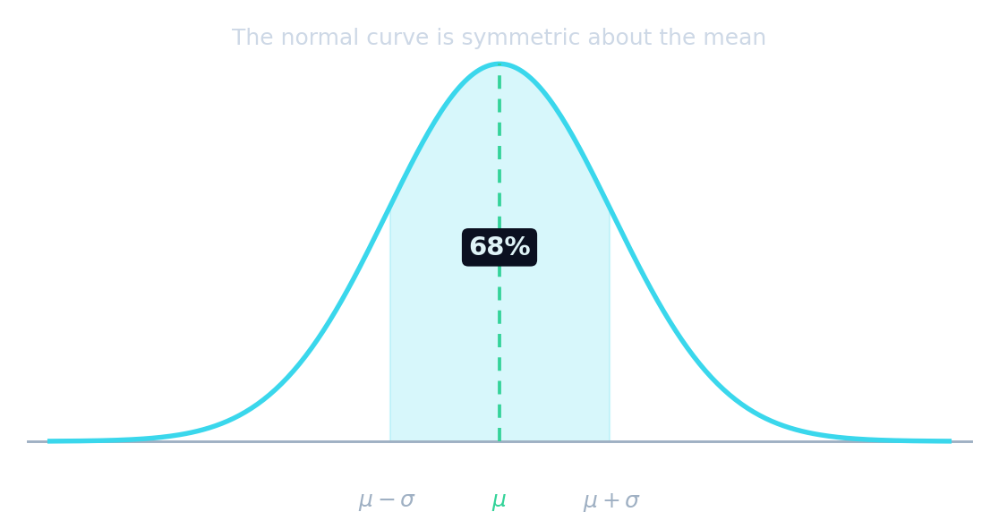
La courbe normale est symétrique par rapport à la moyenne ; environ 68 % de la surface se trouve dans un écart-type.
The normal curve · La courbe normale
P(Z < z)
The · Le area · aire under the bell up to z is the probability · probabilité P(Z < z) — slide z to read it off. · L'aire sous la cloche jusqu'à z est la probabilité P(Z < z) — faites glisser z pour la lire.
The normal distribution curve is: · La courbe de la loi normale est :
It is the symmetric bell-shaped curve centred on the mean μ. · C'est la courbe en cloche symétrique centrée sur la moyenne μ.
Approximately what percentage of values lie within 1 standard deviation of the mean? · Approximativement quel pourcentage de valeurs se trouve dans 1 écart-type de la moyenne ?
The 68-95-99.7 rule: ~68% within 1σ, ~95% within 2σ, ~99.7% within 3σ. · La règle 68-95-99.7 : ~68% dans 1σ, ~95% dans 2σ, ~99.7% dans 3σ.
Complete the standardising formula: Z = (X − μ) / ______. · Complétez la formule de standardisation : Z = (X − μ) / ______.
Z = (X − μ)/σ converts any normal variable to the standard normal N(0, 1). · Z = (X − μ)/σ convertit toute variable normale en la loi normale standard N(0, 1).
Standardising
- To use the tables, standardize 标准化 to $Z \sim N(0, 1)$:
- Then $P(X < x) = P\!\left(Z < \dfrac{x - \mu}{\sigma}\right)$, read from the $\Phi$ table.
A Galton board: balls fall through rows of pegs and pile up into the bell-shaped normal distribution
Standardisation
- Pour utiliser les tableaux, standardisez 标准化 vers $Z \sim N(0, 1)$ :
- Puis $P(X < x) = P\!\left(Z < \dfrac{x - \mu}{\sigma}\right)$, lu dans le tableau $\Phi$.

Un plateau de Galton : des billes tombent à travers des rangées de piquets et s'empilent dans la distribution normale en forme de cloche
X ~ N(50, 4) means μ = 50, σ = 2. Standardize x = 56: what is Z = (x − μ)/σ? · X ~ N(50, 4) signifie μ = 50, σ = 2. Standardisez x = 56 : quelle est Z = (x − μ)/σ ?
Z = (56 − 50)/2 = 6/2 = 3.
X ~ N(100, 25) means μ = 100, σ = 5. Standardize x = 90: Z = (90 − 100)/5. Find Z. · X ~ N(100, 25) signifie μ = 100, σ = 5. Standardisez x = 90 : Z = (90 − 100)/5. Trouvez Z.
Z = (90 − 100)/5 = −10/5 = −2.
Worked example
- $X \sim N(50, 16)$ (so $\mu = 50$, $\sigma = 4$). Find $P(X < 58)$.
- $Z = \dfrac{58 - 50}{4} = 2$.
- $P(Z < 2) = \Phi(2) = 0.9772$.
Standardise before using tables. The $\Phi$ table only works for $Z \sim N(0, 1)$. You must convert $X$ to $Z$ first using $Z = \dfrac{X - \mu}{\sigma}$.
A Galton board produces the bell-shaped normal distribution
Exemple résolu
- $X \sim N(50, 16)$ (donc $\mu = 50$, $\sigma = 4$). Calculez $P(X < 58)$.
- $Z = \dfrac{58 - 50}{4} = 2$.
- $P(Z < 2) = \Phi(2) = 0.9772$.
Standardisez avant d'utiliser les tableaux. Le tableau $\Phi$ ne fonctionne que pour $Z \sim N(0, 1)$. Vous devez convertir $X$ en $Z$ d'abord avec $Z = \dfrac{X - \mu}{\sigma}$.

Un plateau de Galton produit la distribution normale en forme de cloche
If Z = 2, Φ(2) = 0.9772. What is P(Z < 2) (to 4 dp)? · Si Z = 2, Φ(2) = 0.9772. Quelle est P(Z < 2) (à 4 décimales) ?
P(Z < 2) = Φ(2) = 0.9772 from the standard normal table. · P(Z < 2) = Φ(2) = 0.9772 selon la table de la loi normale standard.
Approximating 近似 the binomial
- For large $n$, the normal distribution approximates the binomial: $B(n, p) \approx N(np, np(1-p))$.
- Because you replace a discrete variable by a continuous one, apply a continuity correction 连续性校正 (adjust by 0.5).
For large n the binomial bars closely follow the smooth normal curve N(np, np(1−p))
The binomial distribution B(10, 0.3); its mean is np = 3
- The normal models a continuous random variable; use standardisation $Z=(X-\mu)/\sigma$, and as an approximation to the binomial.
Approximation 近似 de la binomiale
- Pour un grand $n$, la distribution normale approxime la binomiale : $B(n, p) \approx N(np, np(1-p))$.
- Parce que vous remplacez une variable discrète par une variable continue, appliquez une correction de continuité (ajustez de 0.5).
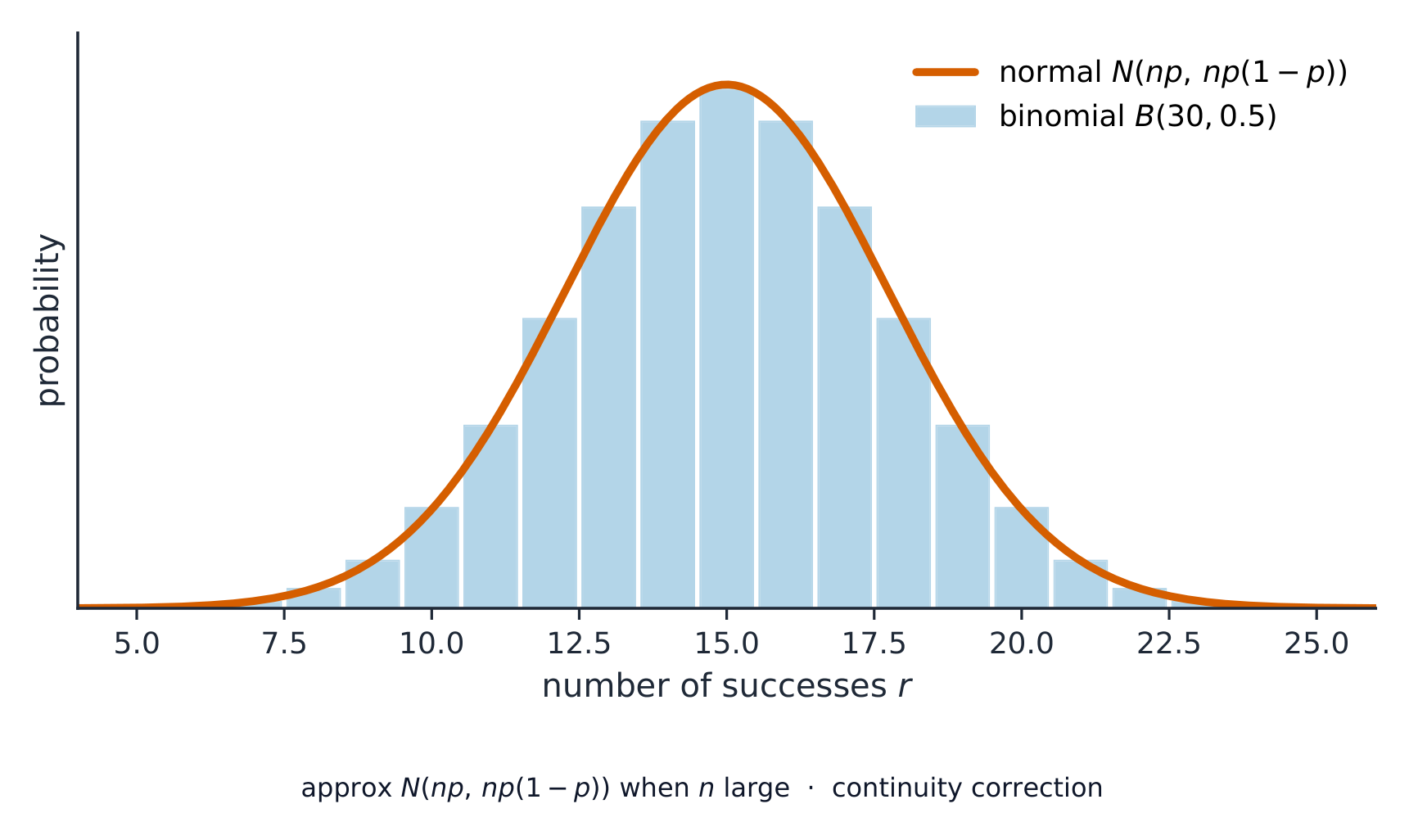
Pour un grand n, les barres binomiales suivent étroitement la courbe normale lisse N(np, np(1−p))
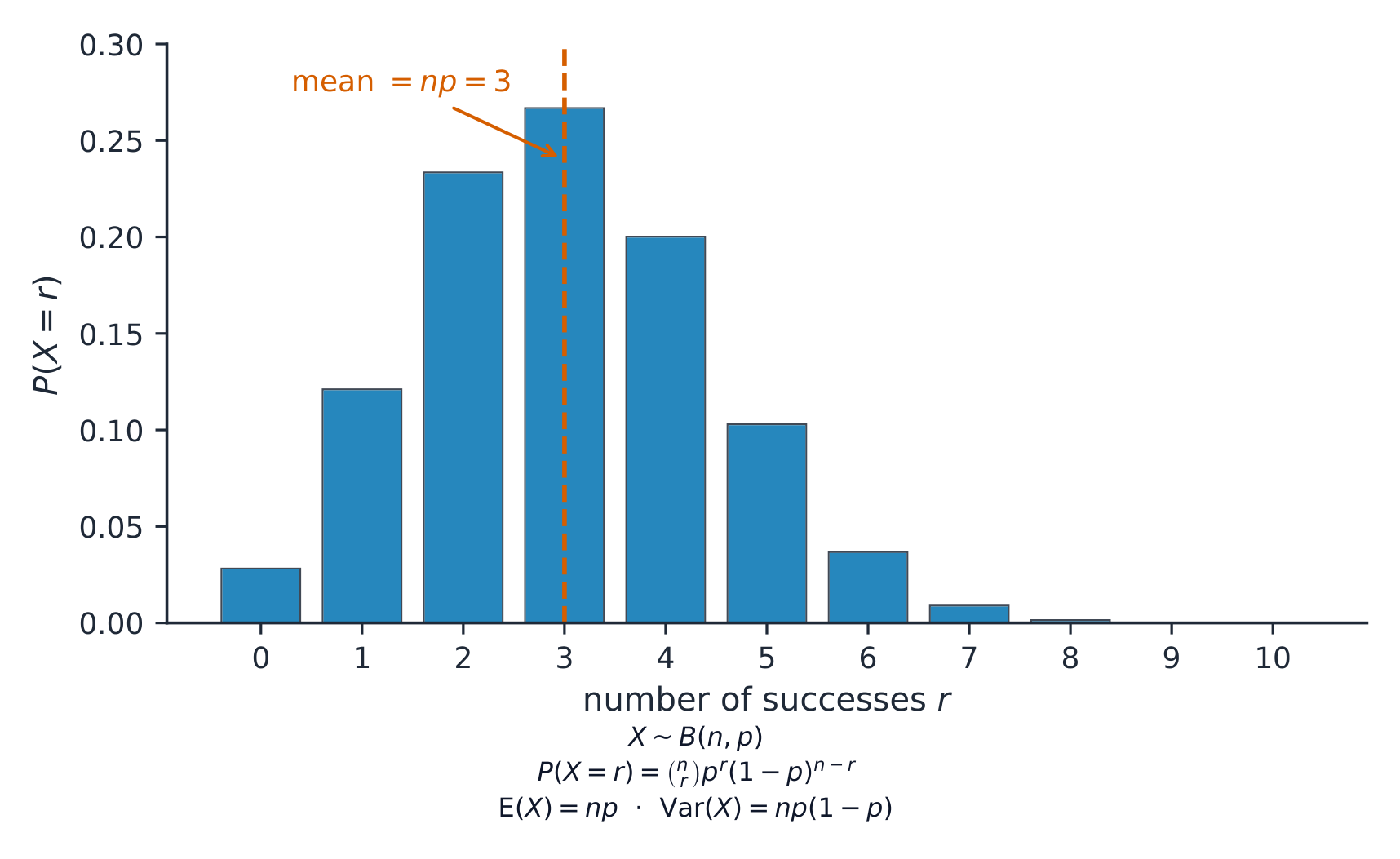
La loi binomiale B(10, 0.3) ; sa moyenne est np = 3
- La normale modélise une variable aléatoire continue ; utilisez la standardisation $Z=(X-\mu)/\sigma$, et comme approximation de la binomiale.
When the normal distribution approximates the binomial, a continuity correction of 0.5 is applied. · Lorsque la loi normale approxime la loi binomiale, une correction de continuité de 0.5 est appliquée.
Replacing a discrete variable with a continuous one needs a ±0.5 continuity correction. · Remplacer une variable discrète par une continue nécessite une correction de continuité ±0.5.
You've got it
- $X \sim N(\mu, \sigma^2)$; standardize with $Z = \dfrac{X - \mu}{\sigma}$
- read probabilities as areas from the $\Phi$ table for $Z \sim N(0,1)$
- the normal approximates the binomial for large $n$ (use a continuity correction)
Vous avez compris
- $X \sim N(\mu, \sigma^2)$ ; standardisez avec $Z = \dfrac{X - \mu}{\sigma}$
- lisez les probabilités comme des surfaces depuis le tableau $\Phi$ pour $Z \sim N(0,1)$
- la normale approxime la binomiale pour un grand $n$ (utilisez une correction de continuité)