Sampling Distribution of x-bar
Introducido| English | Significado |
|---|---|
| sample mean/ˈsæmpl miːn/ | media muestral |
| standard error/ˈstændəd ˈerə/ | error estándar |
One commuter vs fifty commuters
- Commute times in a city are skewed right: most people take 15–35 minutes, a few take over an hour. Can you say how likely one commuter is to take more than 31 minutes? Not without knowing the shape. But the mean of 50 commuters is much more predictable. This lesson explains why.
- A sample mean 样本均值 $\bar{x}$ estimates the population mean $\mu$. Its sampling distribution is centred at $\mu$: $\mu_{\bar{x}}=\mu$, so $\bar{x}$ is an unbiased estimator. Different samples give different $\bar{x}$ values, but they cluster around $\mu$, more tightly for larger $n$.
The standard deviation of $\bar{x}$
- Means vary less than individual values, and less for bigger samples. Because of the square root, quadrupling $n$ halves the spread. When $\sigma$ is unknown, the estimate $s/\sqrt{n}$ is called the standard error 标准误.
- The formula needs independent observations. When sampling without replacement, check the 10% condition: $n\le0.10N$.
Population σ = 20, n = 25. Find the SD of x-bar, σ/√n.
Dificultad 2/5 · 140 monedas + un pequeño bono en el primer intento de hoy
20/√25 = 20/5 = 4.
The standard deviation of the sample mean is...
Dificultad 1/5 · 100 monedas + un pequeño bono en el primer intento de hoy
Divide σ by √n — not by n.
To make the sampling distribution of x-bar have half the spread, you should...
Dificultad 1/5 · 100 monedas + un pequeño bono en el primer intento de hoy
Spread ∝ 1/√n, so 4× n halves the SD.
A population has $\sigma=12$. What sample size makes $\sigma_{\bar{x}}=2$?
Dificultad 2/5 · 140 monedas + un pequeño bono en el primer intento de hoy
$12/\sqrt{n}=2$, so $\sqrt{n}=6$ y $n=36$.
Shape: normal population or the CLT
- If the population is normal, the sampling distribution of $\bar{x}$ is exactly normal for any $n$.
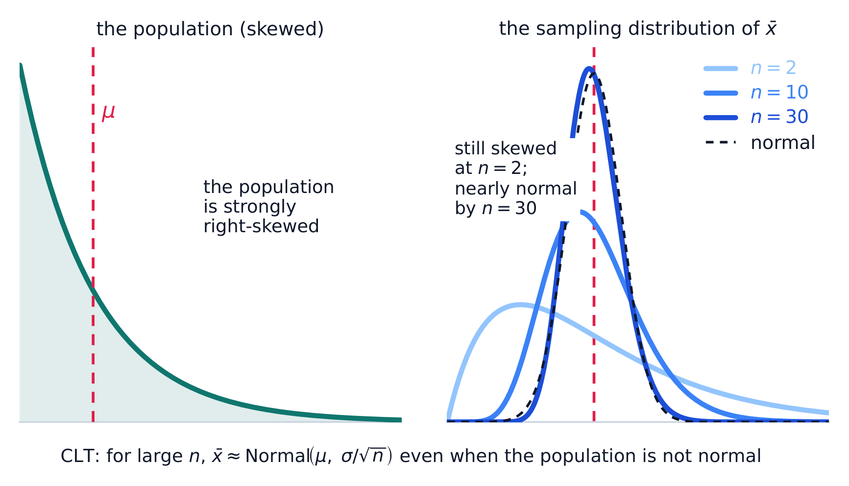
- If not, the Central Limit Theorem 中心极限定理 says $\bar{x}$ is approximately normal when $n$ is large: $n\ge30$ is the usual guideline (strong skew or outliers may need more). For a small sample from a skewed population, you cannot use a normal model.
If the population is already normal, x-bar is normal for any sample size n.
Dificultad 1/5 · 100 monedas + un pequeño bono en el primer intento de hoy
A normal population gives an exactly normal x-bar at any n.
The amounts customers spend at a café are strongly skewed right. In which case is a normal model for $\bar{x}$ most appropriate?
Dificultad 1/5 · 100 monedas + un pequeño bono en el primer intento de hoy
With $n=60\ge30$ the CLT applies. $n=8$ is too small for a skewed population, one customer is not a mean, and the Monday sample is not random.
Probabilities for $\bar{x}$
- Once normality is justified, standardize with the spread of $\bar{x}$, not of individuals: $z=\dfrac{\bar{x}-\mu}{\sigma/\sqrt{n}}$, then use the standard normal table or normalcdf.
- This answers questions like "how unusual is a sample mean this far from $\mu$?", the idea behind every test about means.
$n=25$ from a normal population with $\mu=100$, $\sigma=20$: $\sigma_{\bar{x}}=20/\sqrt{25}=4$. $P(\bar{x}>108)$: $z=(108-100)/4=2$, so $P\approx$ 0.023: a sample mean above 108 is unusual.
With μ=100 and SD of x-bar = 4, find the z-score of x-bar = 108.
Dificultad 2/5 · 140 monedas + un pequeño bono en el primer intento de hoy
z = (108 − 100)/4 = 2.
Use $\sigma/\sqrt{n}$, not $\sigma$, for the spread of $\bar{x}$ — the sample mean varies far less than individual data values. A frequent error is dividing by $n$ instead of $\sqrt{n}$. And justify normality explicitly: either a normal population or the CLT with a large $n$ — don't assume $\bar{x}$ is normal for a small sample from a skewed population.
Battery lifetimes have $\mu=500$ hours and $\sigma=40$ hours (shape unknown). For a random sample of 64 batteries, find $P(\bar{x}<490)$. Give 4 decimal places.
Dificultad 2/5 · 140 monedas + un pequeño bono en el primer intento de hoy
$\sigma_{\bar{x}}=40/\sqrt{64}=5$; CLT applies since $n=64\ge30$. $z=(490-500)/5=-2$, so $P\approx0.0228$.
Worked FRQ: a skewed population
Commute times have mean $\mu=28$ min and SD $\sigma=15$ min, and the distribution is strongly skewed right. A random sample of 50 commuters is taken from the city's 400 000 workers.
(A) Can you find the probability that one randomly chosen commuter takes more than 31 minutes? Explain. No. The population is skewed right, so a normal model is not appropriate for one individual, and we do not know its exact shape.
(B) Describe the sampling distribution of $\bar{x}$. Centre: $\mu_{\bar{x}}=28$ min. Spread: $\sigma_{\bar{x}}=\dfrac{15}{\sqrt{50}}\approx2.12$ min ($50<10\%$ of 400 000, so the formula applies). Shape: approximately normal by the Central Limit Theorem, because $n=50\ge30$.
(C) Find $P(\bar{x}>31)$. $z=\dfrac{31-28}{2.12}\approx1.41$, so $P(\bar{x}>31)\approx$ 0.079.
- Why it scores: (A) separates individuals (need the population shape) from means (CLT). (B) gives centre, spread and shape, each with its reason. (C) names the distribution and shows the $z$-score or the calculator inputs (normalcdf, lower 31, upper ∞, mean 28, SD 2.12).
Individual spread and sample-mean spread
$\mathrm{SD}(\bar X)=\sigma/\sqrt n$
Changing n changes the standard error, not the population standard deviation. Normal probabilities require an explicit distribution model.
The sample mean $\bar{x}$ has $\mu_{\bar{x}} = \mu$ and $\sigma_{\bar{x}} = \frac{\sigma}{\sqrt{n}}$. Justify a normal model either by a normal population or by the Central Limit Theorem ($n\ge 30$); check the 10% condition when sampling without replacement, then find probabilities via $z = \frac{\bar{x}-\mu}{\sigma/\sqrt{n}}$.