The normal distribution · La distribución normal
| English | Español |
|---|---|
| normal distribution/ˈnɔːml ˌdɪstrɪˈbjuːʃn/ | distribución normal |
| continuous variable/kənˈtɪnjuːəs ˈveərɪəbl/ | variable continua |
| standardize/ˈstændədaɪz/ | estandarizar |
| approximate/əˈprɒksɪmət/ | aproximar |
| continuity correction/kɒntɪˈnjuːɪti kəˈrekʃn/ | corrección de continuidad |
The curve that rules the world
- Heights, IQ scores, measurement errors, exam results — all follow the same symmetric bell-shaped curve.
- The normal distribution 正态分布 is the most important distribution in statistics. Master it and you can model almost any continuous variable 连续变量.
La curva que rige el mundo
- Alturas, puntuaciones de CI, errores de medición, resultados de exámenes: todos siguen la misma curva simétrica en forma de campana.
- La distribución normal 正态分布 es la distribución más importante en estadística. Domínala y podrás modelar casi cualquier variable continua 连续变量.
The normal distribution
- The normal distribution models a continuous variable with a symmetric bell shape: $X \sim N(\mu, \sigma^2)$.
- The mean $\mu$ determines the centre; the standard deviation $\sigma$ determines the spread.
The 68-95-99.7 rule. About 68% of values lie within 1 standard deviation of the mean, 95% within 2, and 99.7% within 3.
The normal curve is symmetric about the mean; about 68% of the area lies within one standard deviation.
La distribución normal
- La distribución normal modela una variable continua con una forma simétrica de campana: $X \sim N(\mu, \sigma^2)$.
- La media $\mu$ determina el centro; la desviación estándar $\sigma$ determina la dispersión.
La regla del 68-95-99.7. Aproximadamente el 68% de los valores se encuentran dentro de 1 desviación estándar de la media, el 95% dentro de 2, y el 99.7% dentro de 3.
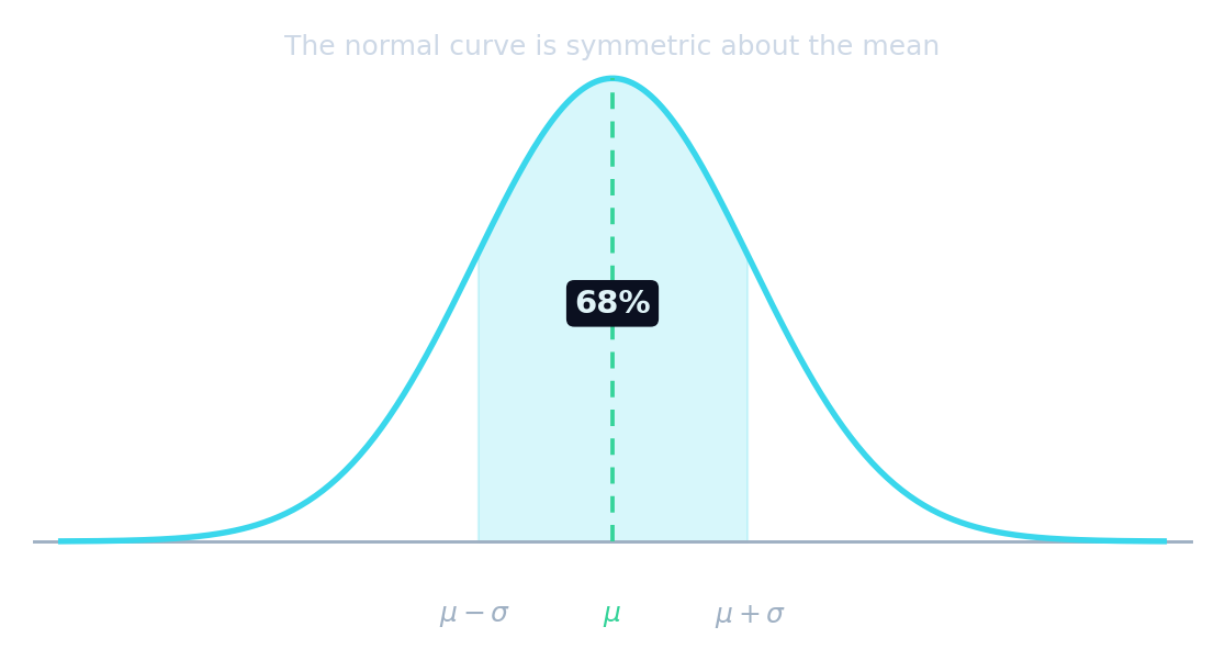
La curva normal es simétrica respecto a la media; aproximadamente el 68% del área se encuentra dentro de una desviación estándar.
The normal curve · La curva normal
P(Z < z)
The · El area · área under the bell up to z is the probability · probabilidad P(Z < z) — slide z to read it off. · El área bajo la campana hasta z es la probabilidad P(Z < z) — desliza z para leerla.
The normal distribution curve is: · La curva de la distribución normal es:
It is the symmetric bell-shaped curve centred on the mean μ. · Es la curva en forma de campana simétrica centrada en la media μ.
Approximately what percentage of values lie within 1 standard deviation of the mean? · Aproximadamente, ¿qué porcentaje de valores se encuentra dentro de 1 desviación estándar de la media?
The 68-95-99.7 rule: ~68% within 1σ, ~95% within 2σ, ~99.7% within 3σ. · Regla 68-95-99.7: ~68% dentro de 1σ, ~95% dentro de 2σ, ~99.7% dentro de 3σ.
Complete the standardising formula: Z = (X − μ) / ______. · Complete la fórmula de estandarización: Z = (X − μ) / ______.
Z = (X − μ)/σ converts any normal variable to the standard normal N(0, 1). · Z = (X − μ)/σ convierte cualquier variable normal a la normal estándar N(0, 1).
Standardising
- To use the tables, standardize 标准化 to $Z \sim N(0, 1)$:
- Then $P(X < x) = P\!\left(Z < \dfrac{x - \mu}{\sigma}\right)$, read from the $\Phi$ table.
A Galton board: balls fall through rows of pegs and pile up into the bell-shaped normal distribution
Estandarización
- Para usar las tablas, estandariza 标准化 para obtener $Z \sim N(0, 1)$:
- Luego $P(X < x) = P\!\left(Z < \dfrac{x - \mu}{\sigma}\right)$, lee desde la tabla $\Phi$.

Un tablero de Galton: las bolas caen a través de filas de clavos y se acumulan formando la distribución normal en forma de campana
X ~ N(50, 4) means μ = 50, σ = 2. Standardize x = 56: what is Z = (x − μ)/σ? · X ~ N(50, 4) significa μ = 50, σ = 2. Estandarice x = 56: ¿cuál es Z = (x − μ)/σ?
Z = (56 − 50)/2 = 6/2 = 3.
X ~ N(100, 25) means μ = 100, σ = 5. Standardize x = 90: Z = (90 − 100)/5. Find Z. · X ~ N(100, 25) significa μ = 100, σ = 5. Estandarice x = 90: Z = (90 − 100)/5. Encuentre Z.
Z = (90 − 100)/5 = −10/5 = −2.
Worked example
- $X \sim N(50, 16)$ (so $\mu = 50$, $\sigma = 4$). Find $P(X < 58)$.
- $Z = \dfrac{58 - 50}{4} = 2$.
- $P(Z < 2) = \Phi(2) = 0.9772$.
Standardise before using tables. The $\Phi$ table only works for $Z \sim N(0, 1)$. You must convert $X$ to $Z$ first using $Z = \dfrac{X - \mu}{\sigma}$.
A Galton board produces the bell-shaped normal distribution
Ejemplo resuelto
- $X \sim N(50, 16)$ (por lo tanto $\mu = 50$, $\sigma = 4$). Encuentra $P(X < 58)$.
- $Z = \dfrac{58 - 50}{4} = 2$.
- $P(Z < 2) = \Phi(2) = 0.9772$.
Estandariza antes de usar las tablas. La tabla $\Phi$ solo funciona para $Z \sim N(0, 1)$. Debes convertir $X$ a $Z$ primero usando $Z = \dfrac{X - \mu}{\sigma}$.

Un tablero de Galton produce la distribución normal en forma de campana
If Z = 2, Φ(2) = 0.9772. What is P(Z < 2) (to 4 dp)? · Si Z = 2, Φ(2) = 0.9772. ¿Cuál es P(Z < 2) (con 4 decimales)?
P(Z < 2) = Φ(2) = 0.9772 from the standard normal table. · P(Z < 2) = Φ(2) = 0.9772 según la tabla de la normal estándar.
Approximating 近似 the binomial
- For large $n$, the normal distribution approximates the binomial: $B(n, p) \approx N(np, np(1-p))$.
- Because you replace a discrete variable by a continuous one, apply a continuity correction 连续性校正 (adjust by 0.5).
For large n the binomial bars closely follow the smooth normal curve N(np, np(1−p))
The binomial distribution B(10, 0.3); its mean is np = 3
- The normal models a continuous random variable; use standardisation $Z=(X-\mu)/\sigma$, and as an approximation to the binomial.
Aproximando 近似 la binomial
- Para $n$ grandes, la distribución normal aproxima la binomial: $B(n, p) \approx N(np, np(1-p))$.
- Dado que reemplazas una variable discreta por una continua, aplica una corrección de continuidad 连续性校正 (ajusta por 0.5).
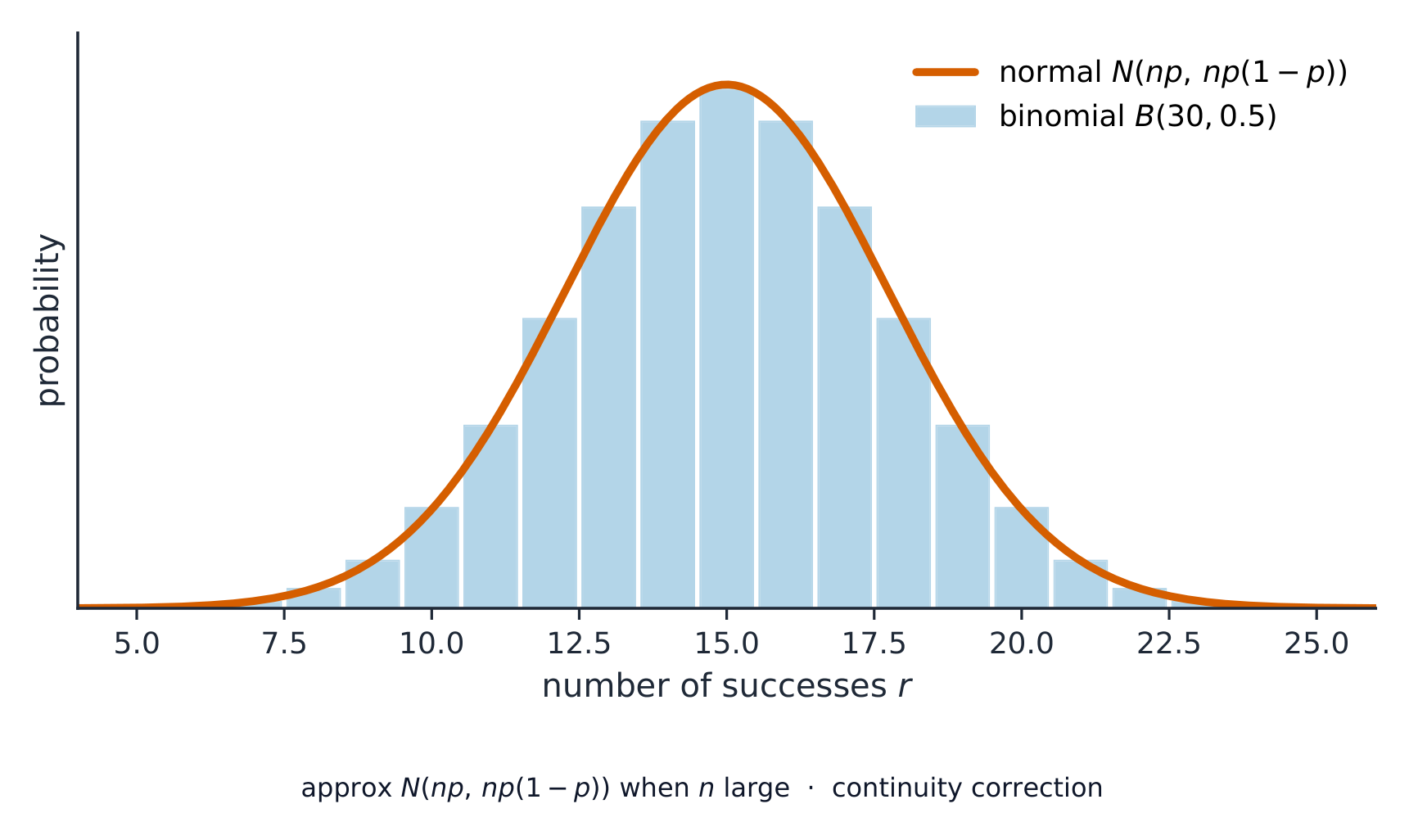
Para n grande, las barras de la binomial siguen de cerca la suave curva normal N(np, np(1−p))
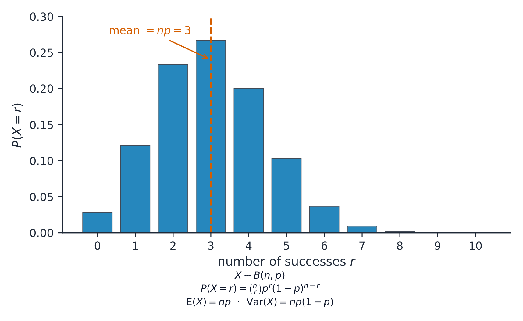
La distribución binomial B(10, 0.3); su media es np = 3
- La normal modela una variable aleatoria continua; usa estandarización $Z=(X-\mu)/\sigma$, y como aproximación a la binomial.
When the normal distribution approximates the binomial, a continuity correction of 0.5 is applied. · Cuando la distribución normal aproxima a la binomial, se aplica una corrección de continuidad de 0.5.
Replacing a discrete variable with a continuous one needs a ±0.5 continuity correction. · Reemplazar una variable discreta por una continua requiere una corrección de continuidad de ±0.5.
You've got it
- $X \sim N(\mu, \sigma^2)$; standardize with $Z = \dfrac{X - \mu}{\sigma}$
- read probabilities as areas from the $\Phi$ table for $Z \sim N(0,1)$
- the normal approximates the binomial for large $n$ (use a continuity correction)
Lo has entendido
- $X \sim N(\mu, \sigma^2)$; normalizar con $Z = \dfrac{X - \mu}{\sigma}$
- leer probabilidades como áreas de la tabla de $\Phi$ para $Z \sim N(0,1)$
- la normal aproxima a la binomial para grandes $n$ (usar una corrección por continuidad)