Differential equations (Further Pure 2) · Ecuaciones diferenciales (Matemáticas Puras Avanzadas 2)
| English | Español |
|---|---|
| differential equation/ˌdɪfəˈrenʃl ɪˈkweɪʒn/ | ecuación diferencial |
| integrating factor/ˈɪntɪɡreɪtɪŋ ˈfæktə/ | factor integrante |
| general solution/ˈdʒenərəl səˈluːʃn/ | solución general |
| complementary function/ˌkɒmplɪˈmentəri ˈfʌŋkʃn/ | función complementaria |
| auxiliary equation/ɔːkˈsɪlɪəri ɪˈkweɪʒn/ | ecuación auxiliar |
| boundary condition/ˈbaʊndəri kənˈdɪʃn/ | condición de contorno |
| initial condition/ɪˈnɪʃl kənˈdɪʃn/ | condición inicial |
| particular integral/pəˈtɪkjʊlə ˈɪntɪɡrəl/ | integral particular |
When the unknown is a function
- Ordinary equations solve for a number. A differential equation 微分方程 solves for a whole function — given a rule about its rate of change.
- They model cooling coffee, growing populations, charging capacitors, and swinging pendulums.
Cuando la incógnita es una función
- Las ecuaciones ordinarias resuelven para un número. Una ecuación diferencial 微分方程 resuelve para una función entera — dado una regla sobre su tasa de cambio.
- Modelan café enfriándose, poblaciones en crecimiento, condensadores cargándose y péndulos oscilando.
First-order linear: the integrating factor 积分因子
- For $\dfrac{dy}{dx} + P(x)\,y = Q(x)$, multiply through by the integrating factor:
- This makes the left side collapse to $\dfrac{d}{dx}(\mu y)$, so you can integrate both sides directly.
Worked example. $\dfrac{dy}{dx} + 2y = e^x$. Here $P = 2$, so $\mu = e^{\int 2\,dx} = e^{2x}$. The left side becomes $\dfrac{d}{dx}(e^{2x}y)$.
Primer orden lineal: el factor integrante 积分因子
- Para $\dfrac{dy}{dx} + P(x)\,y = Q(x)$, multiplique toda la expresión por el factor integrante:
- Esto hace que el lado izquierdo se simplifique a $\dfrac{d}{dx}(\mu y)$, permitiendo integrar ambos lados directamente.
Ejemplo resuelto. $\dfrac{dy}{dx} + 2y = e^x$. Aquí $P = 2$, por lo tanto $\mu = e^{\int 2\,dx} = e^{2x}$. El lado izquierdo se convierte en $\dfrac{d}{dx}(e^{2x}y)$.
Differential equations · Ecuaciones diferenciales
dy/dx = a y
The equation sets the slope · pendiente everywhere; the solution follows those slopes. · La ecuación establece la pendiente en todos lados; la solución sigue esas pendientes.
For dy/dx + 2y = eˣ, the integrating factor μ = e^(∫2 dx) is: · Para dy/dx + 2y = eˣ, el factor integrante μ = e^(∫2 dx) es:
∫2 dx = 2x, so μ = e^(2x). · ∫2 dx = 2x, por lo tanto μ = e^(2x).
Multiplying by the integrating factor makes the left side d/dx(μy), so you can integrate directly. · Multiplicar por el factor integrante hace que el lado izquierdo sea d/dx(μy), por lo que se puede integrar directamente.
That is the whole point of the integrating factor — it makes the left side an exact derivative. · Ese es todo el punto del factor integrante: hace que el lado izquierdo sea una derivada exacta.
Second-order, constant coefficients
- For $a\dfrac{d^2y}{dx^2} + b\dfrac{dy}{dx} + cy = f(x)$, the general solution 通解 has two parts:
- The complementary function 余函数 (CF) comes from the auxiliary equation 辅助方程 $am^2 + bm + c = 0$.
Segundo orden, coeficientes constantes
- Para $a\dfrac{d^2y}{dx^2} + b\dfrac{dy}{dx} + cy = f(x)$, la solución general 通解 tiene dos partes:
- La función complementaria 余函数 proviene de la ecuación auxiliar 辅助方程 $am^2 + bm + c = 0$.
For a constant-coefficient linear equation, the general solution is: · Para una ecuación lineal de coeficientes constantes, la solución general es:
General solution = complementary function (RHS = 0) + a particular integral. · Solución general = función complementaria (RHS = 0) + una integral particular.
Reading the auxiliary roots
- The roots of the auxiliary equation decide the shape of the CF:
| roots | complementary function |
|---|---|
| real & distinct $m_1, m_2$ | $Ae^{m_1 x} + Be^{m_2 x}$ |
| repeated $m$ | $(A + Bx)e^{mx}$ |
| complex $p \pm qi$ | $e^{px}(A\cos qx + B\sin qx)$ |
A differential equation has a whole family of solution curves; the boundary conditions 边界条件 pick out one.
Interpretación de las raíces auxiliares
- Las raíces de la ecuación auxiliar determinan la forma de la función complementaria:
| raíces | función complementaria |
|---|---|
| reales y distintas $m_1, m_2$ | $Ae^{m_1 x} + Be^{m_2 x}$ |
| repetidas $m$ | $(A + Bx)e^{mx}$ |
| complejas $p \pm qi$ | $e^{px}(A\cos qx + B\sin qx)$ |
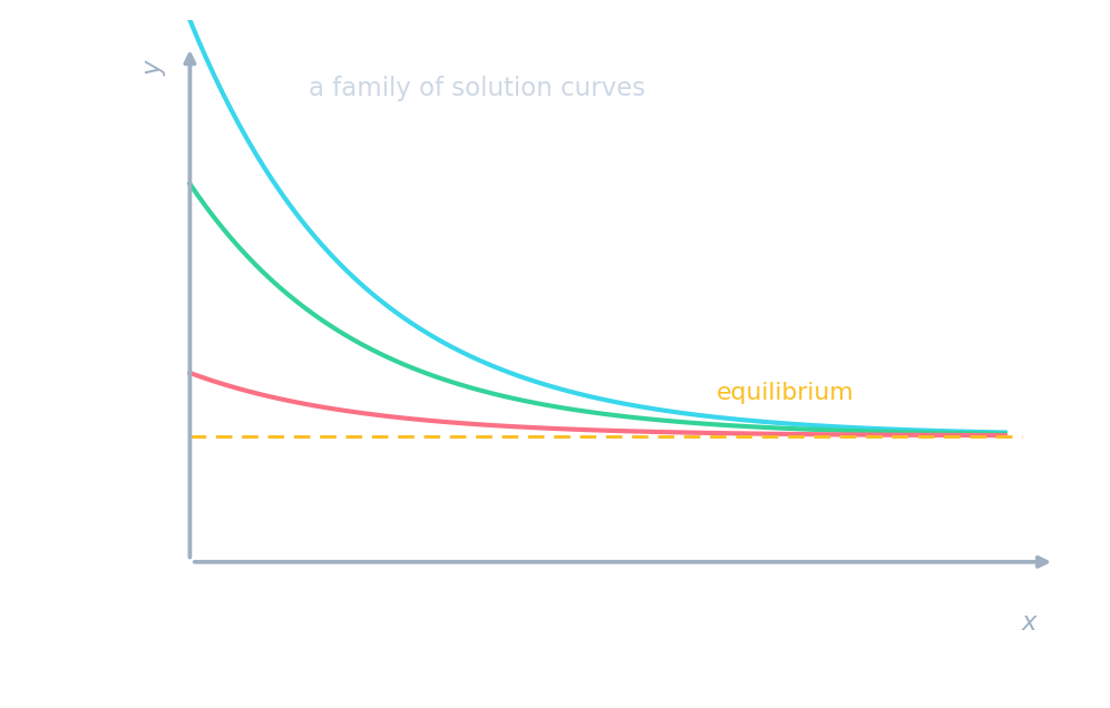
Una ecuación diferencial posee una familia entera de curvas de solución; las condiciones de frontera 边界条件 seleccionan una.
For y″ − 5y′ + 6y = 0 the auxiliary equation is m² − 5m + 6 = 0. What is its larger root? · Para y″ − 5y′ + 6y = 0 la ecuación auxiliar es m² − 5m + 6 = 0. ¿Cuál es su raíz mayor?
m² − 5m + 6 = (m − 2)(m − 3) = 0, so m = 2 or 3; the larger is 3. · m² − 5m + 6 = (m − 2)(m − 3) = 0, por lo que m = 2 o 3; la mayor es 3.
Match each type of auxiliary root to the complementary function it gives. · Asocia cada tipo de raíz auxiliar con la función complementaria que produce.
Distinct reals give two exponentials; a repeated root adds a factor of x; complex roots give an oscillating, exponentially-scaled form. · Los reales distintos dan dos exponenciales; una raíz repetida añade un factor de x; las raíces complejas dan una forma oscilante escalada exponencialmente.
Boundary conditions
- The constants $A, B$ are fixed by boundary or initial conditions 初始条件 (e.g. $y(0) = 1$, $y'(0) = 0$).
- Without them you get the whole family; with them, the one curve that fits.
- Solve differential equations with a substitution or by separable variables, then apply initial conditions for the particular solution.
Condiciones de frontera
- Las constantes $A, B$ se fijan mediante condiciones de frontera o condiciones iniciales 初始条件 (ej. $y(0) = 1$, $y'(0) = 0$).
- Sin ellas se obtiene la familia completa; con ellas, la única curva que se ajusta.
- Resuelva ecuaciones diferenciales mediante una sustitución o por variables separables, y aplique las condiciones iniciales para obtener la solución particular.
The arbitrary constants A and B are fixed by the ______ conditions. · Las constantes arbitrarias A y B se fijan mediante las condiciones ______.
Boundary or initial conditions (like y(0) = 1) determine A and B. · Las condiciones de frontera o iniciales (como y(0) = 1) determinan A y B.
You've got it
- first-order linear: multiply by $\mu = e^{\int P\,dx}$, then integrate
- second-order: general = complementary function + particular integral 特积分
- the CF comes from the auxiliary equation; boundary conditions fix the constants
Ya lo dominas
- primer orden lineal: multiplique por $\mu = e^{\int P\,dx}$, luego integre
- segundo orden: solución general = función complementaria + integral particular 特积分
- la FC proviene de la ecuación auxiliar; las condiciones de frontera fijan las constantes