In this experiment, you will measure the spring constant $k$ of a spring by two different methods.
The spring constant $k$ of a spring is a measure of how difficult the spring is to stretch.
Method 1
• Attach the spring to the clamp, as shown in Fig. 1.1.
- Suspend a mass $m = 500\text{ g}$ from the spring.

- Pull the mass down a small distance (2–3 cm) from its rest position and release it.
The mass oscillates up and down.
The period $T$ of the oscillations is the time taken for one oscillation.
One complete oscillation of the mass is shown in Fig. 1.2.

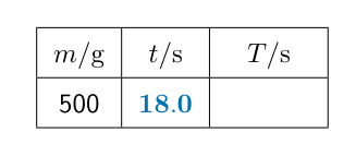
Measure the time $t$ taken for 20 oscillations. Do not remove the mass from the spring.
Record $t$ in Table 1.1.[1]
Table 1.1
| $m/\text{g}$ | $t/\text{ s}$ | $T/\text{ s}$ |
| 500 |
Calculate the period $T$ of the oscillations.
Record your answer in Table 1.1.[1]
Suggest how the procedure can be improved to increase the accuracy of the result.[1]
Calculate a value $k_1$ for the spring constant of the spring.
Use the equation shown. Give your answer to an appropriate number of significant figures.
$k_1 =$ $\text{N/m}$[1]
Method 2
With the 500 g mass still suspended from the spring, measure the stretched length $l$ of the spring in centimetres to the nearest 0.1 cm.
Do not include the loops at the ends of the spring in your measurement.
Record $l$ in Table 1.2.
Table 1.2
| $m/\text{g}$ | $l/\text{cm}$ |
| 500 | |
| 400 | |
| 300 | |
| 200 | |
| 100 |
[1]
Carefully remove the 100 g masses from the mass hanger, one at a time, and repeat the procedure in (b)(i) for $m = 400\text{ g}$, $300\text{ g}$, $200\text{ g}$ and $100\text{ g}$.
Record each value of $l$ in Table 1.2.[1]
Plot a graph of $l/\text{cm}$ ($y$-axis) against $m/\text{g}$ ($x$-axis). Start your axes at the origin $(0,0)$.
Draw the best-fit line.

[3]
Determine the gradient $G$ of your line. Show all working and indicate on the graph the values you use.
$G =$ [1]
An estimated value $k_2$ for the spring constant of the spring can be calculated using the equation
Calculate $k_2$ using your value of $G$ from (b)(iv) and the equation shown.
$k_2 =$ $\text{N/m}$[1]
Two quantities can be considered to be equal within the limits of experimental accuracy if their values are within 10% of each other.
Compare your values of $k_1$ from (a)(iv) and $k_2$ from (b)(v).
State whether your results indicate that the values can be considered to be equal.
Support your statement with a calculation.[2]
[Total: 13]