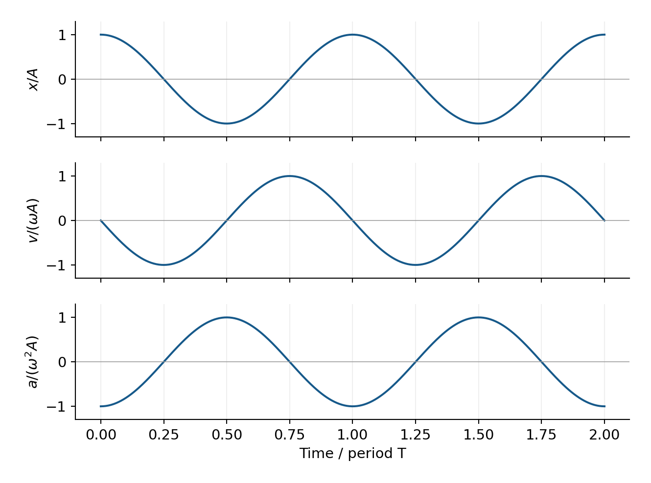
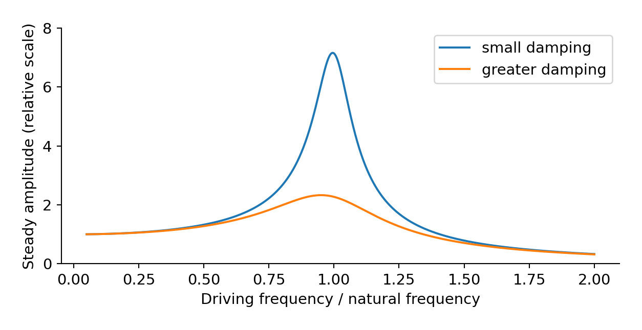
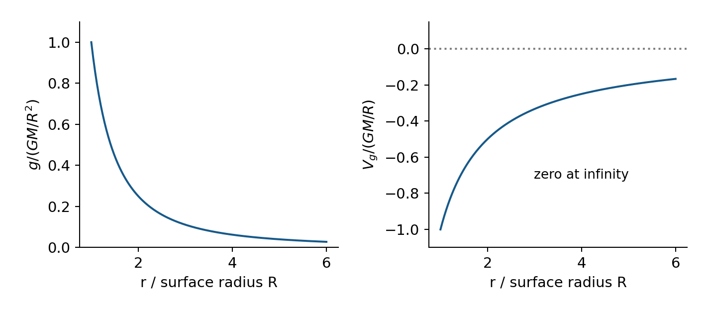
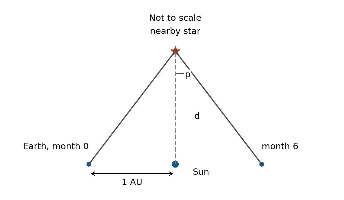
وحدة Edexcel IAL Physics Unit 1 (ورقة WPH11) هي الميكانيكا والمواد: كيف تتحرك الأشياء، وما تفعله القوى، وكيف تتصرف الزخم والطاقة، وكيفية استجابة المواد الصلبة والسائلة للقوى.
الورقة مدتها 1 ساعة و30 دقيقة، وتحتوي على 80 علامة، وكل سؤال إجباري. تمزج بين الاختيار من متعدد والإجابات القصيرة والحسابات وإجابة أو اثنتين من الكتابة الموسعة مُعلمتين بنجمة (*).
على الأقل 32 من 80 العلامات تختبر رياضيات المستوى-2: قراءة الرسوم البيانية، إعادة ترتيب المعادلات، حساب المثلثات والمساحات.
قائمة بالقوانين مطبوعة في نهاية الورقة. احفظ معنى كل رمز ومتى يُسمح باستخدام كل معادلة - القائمة تعطي القوانين، لا الفهم.
استخدم $g = 9.81\ \text{m s}^{-2}$. تتطلب الورقة هذه القيمة؛ استخدام $g = 10$ قد يفقد علامات الدقة. قدم الإجابات النهائية بوحدة وعدد معقول من الأرقام significativa (عادةً 2–3، بما يتوافق مع البيانات).
مقياس السرعة يظهر السرعة عند لحظة واحدة؛ قد تخفي الرحلة توقفات وسرعات. تحل هذه الوحدة رقمًا واحدًا بالصورة الكاملة: الرسوم البيانية والمتجهات والقوى والزخم والطاقة وقوة المواد.
Mechanics and Materials/mɪˈkænɪks ænd məˈtɪərɪəlz/
الميكانيكا والمواد
asterisk/ˈæstərɪsk/
نجمة
trigonometry/ˌtrɪɡəˈnɒmətri/
مثلثات
unit/ˈjuːnɪt/
وحدة
significant figures/sɪɡˈnɪfɪkənt ˈfɪɡəz/
أرقام معنوية
vectors/ˈvektəz/
متجهات
forces/ˈfɔːsɪz/
قوى
momentum/məʊˈmentəm/
الزخم
1.1
الحركة: الكميات والرسوم البيانية
المنهج
وحدة Edexcel IAL للفيزياء 1 (WPH11)، إصدار المواصفة 3 (يوليو 2021)، العبارات 1–3 و11 (التجربة الأساسية 1؛ مرقمة بين عبارات القوة في المواصفة، تُدرَّس هنا مع الحركة).
القدرة على استخدام معادلات الحركة ذات التسارع المنتظم في بُعد واحد: s = (u+v)t/2، v = u + at، s = ut + ½at²، v² = u² + 2as
القدرة على رسم وتفسير بيانات الإزاحة–الزمن، والسرعة–الزمن، والتسارع–الزمن
معرفة الكميات الفيزيائية المستخرجة من ميل ومساحات بيانات الإزاحة–الزمن، والسرعة–الزمن، والتسارع–الزمن، بما في ذلك حالات عدم انتظام التسارع، وفهم كيفية استخدام هذه الكميات
التجربة الأساسية 1: تحديد تسارع جسم يسقط سقوطاً حراً
المصدر: منهج كامبريدج الدولي
الإزاحة — التغير الخطي المستقيم في الموقع، مع الاتجاه (متجه). المسافة — طول المسار الكلي (كمية قياسية، بلا اتجاه).
السرعة المتجهة — معدل تغير الإزاحة. السرعة القياسية — معدل تغير المسافة.
التسارع — معدل تغير السرعة: $a = \dfrac{\Delta v}{\Delta t}$، الوحدة $\text{m s}^{-2}$.
لأن الإزاحة هي الخط المستقيم من البداية إلى النهاية، فإن المسار المنحني يعطي دائمًا المسافة > مقدار الإزاحة - يسأل الممتحن عن هذه المقارنة بالضبط.
قراءة رسوم بيانية الحركة
على الرسم البياني للإزاحة-الزمن، الميل هو السرعة. الخط المنحني يعني سرعة متغيرة؛ خذ ميل الخط المماس عند النقطة.
في منحنى السرعة–الزمن، يمثل الميل التسارع، والمساحة بين الخط ومحور الزمن هي الإزاحة. المساحة تحت المحور تمثل إزاحة سالبة (حركة للخلف)؛ بينما المسافة تُحسب بجمع قيم جميع المساحات.
في منحنى التسارع–الزمن، تمثل المساحة تحت الخط التغير في السرعة.
التسارع الثابت غير الصفرية يحني منحنى الإزاحة–الزمن إلى شكل قطع مكافئ؛ والخط المستقيم على ذلك المنحنى يعني تسارعاً صفراً.
مثال محلول (بنمط يونيو 2025). خط سرعة–زمن يرتفع بشكل مستقيم من $1.8\ \text{m s}^{-1}$ عند $t = 4\ \text{s}$ إلى $5.0\ \text{m s}^{-1}$ عند $t = 16\ \text{s}$.
المعطيات: زوجان $(t, v)$ على الجزء المستقيم. السبب: التسارع هو ميل منحنى السرعة–الزمن.
التحقق: بما أن الخط يرتفع بلطف، فإن تسارعاً صغيراً يعتبر معقولاً.
معادلات سوافات الأربعة
لـتسارع منتظم (تسارع ثابت) في بُعد واحد، مع $s$ إزاحة، $u$ سرعة ابتدائية، $v$ سرعة نهائية، $a$ تسارع، $t$ زمن:
$$v = u + at \qquad s = \frac{(u+v)t}{2} \qquad s = ut + \tfrac{1}{2}at^2 \qquad v^2 = u^2 + 2as$$
اختر المعادلة التي تحتوي على كمياتك المعطاة والمجهولة — ولا شيء لا تعرفه. لا يوجد $t$؟ استخدم $v^2 = u^2 + 2as$. لا يوجد $a$؟ استخدم $s = \tfrac{(u+v)}{2}t$.
هذه المعادلات صالحة فقط طالما كان التسارع ثابتاً. المنحنى المتعرج في منحنى السرعة–الزمن يدل على تسارع متغير؛ لكن المنحنى المتعرج في منحنى الإزاحة–الزمن قد يظل يمثل تسارعاً ثابتاً.
السقوط الحر هو تسارع منتظم مع $a = g = 9.81\ \text{m s}^{-2}$ لأسفل (مع إهمال مقاومة الهواء).
مثال محلول (استنتاج ومقارنة، يونيو 2025 س13). قُذفت كرة سلة من ارتفاع $1.7\ \text{m}$ فوق الأرض بسرعة رأسية ابتدائية $5.1\ \text{m s}^{-1}$ لأعلى، ودخلت الحلقة وهي تتحرك لأسفل بسرعة $2.1\ \text{m s}^{-1}$. هل تقع الحلقة على ارتفاع $3.0\ \text{m}$ فوق الأرض؟
ارتفاع الحلقة $= 1.7\ \text{m} + 1.1\ \text{m} = 2.8\ \text{m} \neq 3.0\ \text{m}$، لذا كانت الحلقة ليست على الارتفاع المعياري. يُكتسب الدرجة الأخيرة فقط في سؤال "استنتج ما إذا" عند ذكر المقارنة والاستنتاج.
التجربة الأساسية 1: قياس $g$
أفلع جسماً وقيسه: باستخدام بوابة ضوئية أو فيديو بمعدل إطارات معروف، احصل على $s$ و$t$ (أو سرعتين عند نقطتين) واستخدم معادلة سوافات. طريقة أكثر نظافة: ارسم $s$ مقابل $t^2$ لـ$s = \tfrac{1}{2}gt^2$ — وهو خط مستقيم يمر بنقطة الأصل بميل $g/2$. يكشف الخط المستقيم الذي لا يمر بنقطة الأصل عن انحراف منهجي، مثل انحراف ثابت في المسافة المقاسة. كما يمكن أن يشوه تأخير في التوقيت العلاقة؛ ويقلل التوقيت الآلي من خطأ وقت الاستجابة. في التصوير بالوميض، يتحرك الجسم أثناء كل وميض. ينتج الوميض الأقصر صورة أوضح ونطاقاً أصغر للمواقع الممكنة، مما يقلل عدم اليقين في قراءة المسافة إذا بقي المقياس ودقة الصورة دون تغيير.
1.2
الكميات القياسية والمتجهة وحركة المقذوفات
المنهج
وحدة Edexcel IAL للفيزياء 1 (WPH11)، إصدار المواصفة 3 (يوليو 2021)، العبارات 4–7.
فهم الكميات القياسية والمتجهة ومعرفة أمثلة على كل نوع من أنواع الكميات والتعرف على رمز المتجه
القدرة على تحليل متجه إلى مركبتين متعامدتين على بعضهما البعض بالرسم وبالعملية الحسابية
القدرة على إيجاد المحصلة لمجموعتي متجهين مستويين بأي زاوية بينهما بالرسم، وبزاوية قائمة بينهما بالعملية الحسابية
فهم كيفية الاستفادة من استقلالية الحركة الرأسية والأفقية لمقذوف يتحرك بحرية تحت تأثير الجاذبية
المصدر: منهج كامبريدج الدولي
المتجه له مقدار واتجاه (الإزاحة، السرعة، التسارع، القوة، الزخم)؛ أما الكمية القياسية فله magnitude فقط (المسافة، السرعة، الشغل، الطاقة). ترميز المتجهات في الورقة يكون بسهم فوق الرمز، $\vec{F}$.
تحليل ودمج
تفكيك متجه إلى مركبتين متعامدتين: المركبة من القوة $F$ عند زاوية $\theta$ في اتجاه معين هي $F\cos\theta$ إذا كانت $\theta$ مقاسة من ذلك الاتجاه، و$F\sin\theta$ من العمودي عليها. اختر برسم المثلث القائم بدلاً من الاعتماد على العادة.
دمج مركبتين متعامدتين يعيد بناء المتجه: المقدار $R = \sqrt{F_x^2 + F_y^2}$، والاتجاه محدد بـ $\tan\theta = F_y / F_x$.
اجمع قبل التربيع. المحصلة لـ $500\ \text{N}$ و$200\ \text{N}$ المتعامدين هي $\sqrt{500^2 + 200^2}\ \text{N}$، وليست $\sqrt{500^2} + \sqrt{200^2}$.
عند أي زاوية، اجمع المتجهات برسم مخطط مقياس (مثلث متجهي، ذيل الرأس إلى الذيل) أو بفصل كل متجه إلى مركباته أولاً. في حالة التوازن، يغلق المثلث المتجهي: $\vec{W} + \vec{T_1} + \vec{T_2} = 0$.
مثال محلول. صندوق مستقر على منحدر بزاوية $\theta$ مع الأفقي، وتؤثر عليه قوة ثقل $W$ رأسياً للأسفل.
السبب: اتجاه الانزلاق يكون موازياً للمنحدر، لذا نفصل $W$ إلى مركبات موازية وعمودية على المنحدر.
عند سرعة ثابتة تكون المحصلة صفراً، لذا تكون قوة الاحتكاك $F = W\sin\theta$ مساوية لها تماماً. (تعمل ⟨$W\cos\theta$⟩ عمودياً على المنحدر وتتوازن مع قوة التماسك).
حركة المقذوفات
المقذوف الذي يتحرك بحرية تحت تأثير الجاذبية هو حركة مستقلة في اتجاهين: سرعة أفقية ثابتة (لا توجد قوة أفقية)، وسرعة رأسية تتغير تحت تأثير $g$.
يعتمد وقت السقوط فقط على الحركة الرأسية. كرةان تتركان طاولة بسرعات مختلفة — أو بكتل مختلفة — تهبطان بعد نفس الوقت: الكتلة والسرعة الأفقية لا تظهران في $s = ut + \tfrac{1}{2}gt^2$.
الطريقة: افكك سرعة الإطلاق إلى مركبة $u_h = u\cos\theta$ ومركبة $u_v = u\sin\theta$؛ طبق معادلات suvat بشكل منفصل لكل اتجاه؛ الزمن يربط بين الحركتين.
مثال محلول (يناير 2025 سؤال 19). يُطلق مقذوف بسرعة $500\ \text{m s}^{-1}$، بزاوية $22^\circ$ فوق الأفقي، من ارتفاع $2.0\ \text{km}$ فوق سطح البحر. أثبت أنه يعبر فوق سفينة تبعد $15\ \text{km}$ بعد حوالي $30\ \text{s}$.
معطيات: $u$، $\theta$، المسافة الأفقية $s_h$. الحركة الأفقية لها $a = 0$، لذا استخدم $s_h = u_h t$.
وحدة Edexcel IAL للفيزياء 1 (WPH11)، إصدار المواصفة 3 (يوليو 2021)، العبارات 8–10 و12 (عبارة 11، التجربة الأساسية 1، تُدرَّس في ورقة 1.1 مع الحركة).
القدرة على رسم وتفسير مخططات القوى الحرة لتمثيل القوى المؤثرة على جسيم أو على جسم ممتد لكن صلب باستخدام مفهوم مركز ثقل الجسم الممتد
القدرة على استخدام المعادلة ΣF = ma، وفهم كيفية استخدامها في الحالات التي يكون فيها m ثابتاً (قانون نيوتن الثاني للحركة)، بما في ذلك قانون نيوتن الأول للحركة حيث a = 0، الأجسام الساكنة أو التي تتحرك بسرعة منتظمة؛ يُتوقع استخدام مصطلح السرعة النهاية
القدرة على استخدام معادلات شدة المجال الجاذبي g = F/m والوزن W = mg
معرفة وفهم قانون نيوتن الثالث للحركة، ومعرفة خصائص أزواج القوى في التفاعل بين جسمين
المصدر: منهج كامبريدج الدولي
مخطط الجسم الحر يعرض فقط القوى المؤثرة على الجسم المختار — ولا يشمل القوى التي يطبقها الجسم على أشياء أخرى. على جسم ممتد، يعمل الوزن عند مركز الثقل.
قانون نيوتن الأول: محصلة القوى صفر تعني عدم تغير الحركة — إما ساكن أو يتحرك بسرعة ثابتة. السرعة الثابتة ليست "عدم وجود قوى"؛ بل هي توازن القوى.
قانون نيوتن الثاني: $\sum F = ma$. القوة المحصلة تسبب التسارع؛ اذكر كل قوة، واختر اتجاهًا موجبًا، ثم طبق القانون.
قانون نيوتن الثالث: عندما يؤثر الجسم A بقوة على الجسم B، يُؤثر B بقوة مساوية وعكسية على A. تعمل الزوجتان على جسمين مختلفين، وهما من نفس النوع، وتعملان على امتداد خط واحد. وزن الكتاب وقوة التلامس العمودية للطاولة ليسا زوج قانون نيوتن الثالث: لأنهما تعملان على نفس الجسم.
الوزن$W = mg$؛ شدة المجال الجاذبي$g = \dfrac{F}{m}$، وبالتالي $g = 9.81\ \text{N kg}^{-1}$.
السرعة الحدية: عندما يزداد سرعة جسم ساقط، تزداد مقاومة الهواء حتى تساوي (مقاومة الهواء + الدفع) الوزن؛ عندها تكون القوة المحصلة صفرًا وتتوقف السرعة عن التغير. مصطلح "حدّي" يشير إلى توازن القوى، وليس حدًا سرعيًا مُثبتًا في الطبيعة.
مثال محلول (يونيو 2025 Q11). قوة محصلة مقدارها $4800\ \text{N}$ تُسرّع قاربًا بمقدار $0.31\ \text{m s}^{-2}$. أوجد وزن القارب.
تحقق: الإجابة تتطلب معادلتين متتاليتين؛ والوحدة هي نيوتن، وليست كيلوجرامات.
1.4
الزخم
المنهج
Edexcel IAL Physics Unit 1 (WPH11)، نسخة المواصفة 3 (يوليو 2021)، العبارات 13–14.
فهم أن الزخم يُعرَّف بالمعادلة p = mv
معرفة مبدأ حفظ الزخم الخطي، وفهم كيفية ربطه بقوانين نيوتن للحركة وتطبيقه على المسائل ذات البعد الواحد
المصدر: منهج كامبريدج الدولي
كمية الحركة$p = mv$، وهي كمية متجهة، ووحدة القياس $\text{kg m s}^{-1}$.
حفظ كمية الحركة الخطية: عندما تكون القوة الخارجية المحصلة صفرًا (أو يكون دافعتها خلال تفاعل قصير مهملاً)، فإن مجموع كميات الحركة قبل الحدث يساوي مجموعها بعد. أعطِ السرعات إشارات: اختر اتجاهًا واحدًا كموجب وأبقه ثابتًا.
ينتج حفظ كمية الحركة من قانوني نيوتن الثاني والثالث: فالقوى المتبادلة بين الجسمين متساوية وعكسية، وتعملان لنفس المدة، لذا تكون التغيرات في كميات الحركة متساوية وعكسية.
الطاقة الحركية قد لا تبقى بعد التصادم، بينما كمية الحركة دائمًا محفوظة (في النظام المعزول).
مثال محلول (يونيو 2025 Q10). قطار كتلته $3m$ يتحرك بسرعة $v$ يصطدم بعربة كتلتها $m$ تتحرك بسرعة $2v$ في الاتجاه المعاكس؛ فيتصلا. أوجد السرعة الجديدة.
معطيات: الكتل والسرعات في اتجاهين متعاكسين. السبب: زوج معزول، لذا نطبق حفظ كمية الحركة بالإشارات. نأخذ اتجاه القطار كاتجاه موجب.
$$p_{\text{before}} = p_{\text{after}}$$
$$3m \times v + m \times (-2v) = (3m + m)\,V$$
$$mv = 4mV \quad\Rightarrow\quad V = \frac{v}{4}$$
تحقق: بما أن كميات الحركة تلغي بعضها تقريبًا، فإن سرعة مجتمعة صغيرة في اتجاه القطار تبدو منطقية.
1.5
العزوم والتوازن
المنهج
Edexcel IAL Physics Unit 1 (WPH11)، نسخة المواصفة 3 (يوليو 2021)، العبارات 15–16.
القدرة على استخدام معادلة عزم القوة: عزم القوة = Fx، حيث x هو المسافة العمودية بين خط عمل القوة ومحور الدوران
القدرة على استخدام مفهوم مركز ثقل جسم ممتد وتطبيق مبدأ العزوم على جسم ممتد في حالة توازن
المصدر: منهج كامبريدج الدولي
عزم القوة حول نقطة ارتكاز هو $\text{moment} = Fx$، حيث $x$ هو المسافة العمودية من نقطة الارتكاز إلى خط عمل القوة. إذا كانت القوة تصادف الرافعة بزاوية $\theta$، استخدم المكون العمودي $F\sin\theta$ أو المسافة العمودية — ولا تستخدم الاثنين معًا.
مبدأ العزوم: في حالة التوازن، مجموع العزوم في الاتجاه عقارب الساعة = مجموع العزوم عكس اتجاه عقارب الساعة (العزم المحصل يساوي صفرًا).
التوازن الكامل يتطلب كلا الشرطين: القوة المحصلة صفر والعزم المحصل صفر. ميزان متذبذب يحمل أطفالًا متساوين عند مسافات متساوية يحقق كلا الشرطين؛ أما الأطفال أنفسهم عند مسافات غير متساوية فيوازن القوى لكنه لا يوازن العزوم.
بالنسبة لعارضة منتظمة، يعمل الوزن في مركزها.
مثال محلول (يونيو 2025 Q19). عارضة مستوية منتظمة طولها $1.40\ \text{m}$ ووزنها $95\ \text{N}$، موضوعة بزاوية $42^\circ$ أفقيًا، مرتكزة عند أحد طرفيها. يدفع مكبس بالعارضة بقوة $160\ \text{N}$ بزاوية $18^\circ$ نسبت إليها، على بُعد $0.37\ \text{m}$ من نقطة الارتكاز. ما هي القوة العمودية $F$ عند مقبض النهاية التي ترفع العارضة فقط؟
معطيات: الهندسة، القوتان، الزاويتان. السبب: الرفع البسيط يعني التوازن عند نقطة الارتكاز، لذا نطبق مبدأ العزوم باستخدام المركبات العمودية.
إذا تم سحب رأسياً من المقبض بدلاً من ذلك: فإن مسافته العمودية إلى نقطة الارتكاز تكون أقصر من طول السكة، مما يستلزم قوة أكبر لتحقيق نفس العزم.
1.6
الشغل والطاقة والقوة والكفاءة
المنهج
Edexcel IAL Physics Unit 1 (WPH11)، نسخة المواصفة 3 (يوليو 2021)، العبارات 17–22.
القدرة على استخدام معادلة الشغل ΔW = FΔs، بما في ذلك الحسابات عندما لا تكون القوة على طول خط الحركة
القدرة على استخدام المعادلة Ek = ½mv² لطاقة الحركة للجسم
القدرة على استخدام المعادلة ΔEgrav = mgΔh للفرق في الطاقة الكامنة الجاذبية بالقرب من سطح الأرض
معرفة كيفية تطبيق مبدأ حفظ الطاقة، بما في ذلك استخدام الشغل المبذول، والطاقة الكامنة الجاذبية، وطاقة الحركة
القدرة على استخدام المعادلات التي تربط بين القدرة والزمن والطاقة المنقولة أو الشغل المبذول P = E/t وP = W/t
القدرة على استخدام معادلات الكفاءة: الكفاءة = الطاقة المفيدة الناتجة / إجمالي الطاقة المدخلة، والكفاءة = القدرة المفيدة الخارجة / إجمالي القدرة الداخلة
المصدر: منهج كامبريدج الدولي
الشغل$\Delta W = F\Delta s$ عندما تؤثر القوة على طول المسار؛ وإذا كانت القوة بزاوية $\theta$ على المسار، فإنها تقوم بالشغل فقط مركبتها الموازية للمسار: $\Delta W = F\Delta s\cos\theta$.
الطاقة الحركية$E_k = \tfrac{1}{2}mv^2$ — مضاعبة السرعة تربع الطاقة.
الطاقة الكامنة الجاذبية$\Delta E_{\text{grav}} = mg\Delta h$ بالقرب من سطح الأرض.
حفظ الطاقة: تنتقل الطاقة أو تتحول، ولا تُخلق ولا تُفنى. في السقوط مع مقاومة الهواء، $\Delta E_{\text{grav}}$ يتحول إلى $E_k$بالإضافة إلى الشغل المبذول ضد مقاومة الهواء؛ وعند السرعة النهائية $E_k$ ثابتة، لذا كل$\Delta E_{\text{grav}}$ يذهب للشغل ضد المقاومة.
القوة (القدرة)$P = \dfrac{E}{t} = \dfrac{W}{t}$ — الطاقة المنتقلة لكل وحدة زمن.
الكفاءة$= \dfrac{\text{useful energy output}}{\text{total energy input}} = \dfrac{\text{useful power output}}{\text{total power input}}$.
مثال محلول (يونيو 2025 Q14). سيارة كهربائية كتلتها $1800\ \text{kg}$ سرعتها $14\ \text{m s}^{-1}$ تتوقف على تلة، وتكتسب ارتفاعاً قدره $0.76\ \text{m}$؛ battery اكتسبت $45\ \text{kJ}$. أوجد كفاءة الفرامل.
معطيات: $m$، $v$، $\Delta h$، مكسب البطارية. السبب: إجمالي المدخل هو الطاقة التي أزالتها الفرامل — الطاقة الحركية المفقودة ناقص الطاقة الكامنة الجاذبية التي احتفظت بها السيارة بسبب ارتفاعها النهائي.
Edexcel IAL Physics Unit 1 (WPH11)، نسخة المواصفة 3 (يوليو 2021)، العبارات 23–26.
القدرة على استخدام معادلة الكثافة ρ = m/V
فهم كيفية استخدام العلاقة: قوة الطفو = وزن السائل المُزاح
أ) القدرة على استخدام معادلة مقاومة اللزوجة (قانون ستوكس) F = 6πηrv؛ ب) فهم أن هذه المعادلة تنطبق فقط على الأجسام الكروية الصغيرة التي تتحرك بسرعات منخفضة مع تدفق طبقي (أو في غياب التدفق المضطرب)، وأن اللزوجة تعتمد على درجة الحرارة
الممارسة العملية الأساسية 2: استخدام طريقة سقوط الكرة لتحديد لزوجة سائل
الدفع الهيدروستاتيكي = وزن السائل المزاح — أي وزن السائل المزاح، وليس حجمه أو كتلته.
قانون ستوكس: مقاومة اللزوجة على كرة صغيرة بسرعة منخفضة في تدفق طبقي هي $F = 6\pi\eta rv$، حيث $\eta$ هي اللزوجة، $r$ نصف القطر، $v$ السرعة. هذا القانون صالح فقط للكرات الصغيرة المتحركة ببطء بدون اضطراب، و$\eta$ ينخفض عندما تسخن السوائل في هذه التجربة؛ الغازات لا تتبع هذا الاتجاه عادةً.
تجربة أساسية 2: قياس اللزوجة بطريقة سقوط الكرة
أسقط كرة محشورة في أسطوانة مدرجة تحتوي على السائل. انتظر حتى تسقط الكرة بسرعة نهائية، ثم قس وقت قطرها لمسافة محددة. عند السرعة النهائية، تتوازن القوى: الوزن = الدفع الهيدروستاتيكي + مقاومة اللزوجة، لذا
تحتاج إلى نصف قطر الكرة وكتلتها (أو كثافتها)، وكثافة الزيت، ومسافة السقوط، والزمن. الزيت الدافئ أقل لزوجة، لذا تسقط الكرة بشكل أسرع ويكون الزمن المقاس أقصر.
be able to use the Hooke's law equation ΔF = kΔx, where k is the stiffness of the object
understand how to use the relationships (tensile or compressive) stress = force / cross-sectional area, (tensile or compressive) strain = change in length / original length, and Young modulus = stress / strain
a) be able to draw and interpret force–extension and force–compression graphs; b) understand the terms limit of proportionality, elastic limit, yield point, elastic deformation and plastic deformation and be able to apply them to these graphs
be able to draw and interpret tensile or compressive stress–strain graphs, and understand the term breaking stress
CORE PRACTICAL 3: Determine the Young modulus of a material
be able to calculate the elastic strain energy Eel in a deformed material sample, using the equation ΔEel = ½FΔx, and from the area under the force–extension graph; the estimation of area and hence energy change for both linear and non-linear force–extension graphs is expected
المصدر: منهج كامبريدج الدولي
قانون هوك: $\Delta F = k\,\Delta x$ طالما تتصرف المادة بشكل طردي؛ $k$ هو الصلابة (ثابت المرونة)، وهو ميل منحنى القوة–الاستطالة.
على منحنى القوة–الاستطالة أو الإجهاد–الانفعال: ينتهي الجزء المستقيم عند حد التناسب؛ وبعيداً عن الحد المرن لا تعود العينة إلى طولها الأصلي (تشوه مرن = يعاود الطول الأصلي؛ تشوه بلاستيكي = يبقى مدوداً)؛ والمادة ذات نقطة خضوع مميزة يمكن أن تمتد بشكل كبير مع زيادة طفيفة في القوة عند الخضوع؛ والمواد اللدنة الأخرى تخضع تدريجياً. تشير نقطة الخضوع إلى بداية التدفق البلاستيكي الكبير؛ وإجهاد الكسر هو الإجهاد عند الانكسار.
طاقة الانفعال المرن: $\Delta E_{\text{el}} = \tfrac{1}{2}F\Delta x$ لزنبرك خطي — وهي المساحة تحت منحنى القوة–الاستطالة. ومنحنى غير خطي، يُقدّر المساحة بالمربعات. المساحة تحت منحنى التحميل الإجهاد–الانفعال هي الشغل المبذول لكل وحدة حجم، لأن $\dfrac{F}{A} \times \dfrac{\Delta x}{x} = \dfrac{F\Delta x}{V}$. وفي المنطقة المرنة تُخزن هذه الطاقة قابل للاسترداد كطاقة انفعال مرن؛ والشغل المبذول خارج الحد المرن ليس كله قابلاً للاسترداد.
مثال محلول (يونيه 2025 Q17b). وتر كمان طوله الأصلي $0.750\ \text{m}$ ونصف قطره $0.85 \times 10^{-3}\ \text{m}$ يتمدد إلى $0.752\ \text{m}$ تحت تأثير قوة $36\ \text{N}$. أوجد معامل يونغ.
معلوم: $F$، $x$، $\Delta x$، $r$. السبب: $E = \sigma/\varepsilon$ يتطلب الإجهاد والانفعال؛ والإجهاد يحتاج مساحة المقطع العرضي.
تحقق: معامل سلك معدني هو $10^{9}$–$10^{12}\ \text{Pa}$؛ $6\ \text{GPa}$ يقع في هذا النطاق.
التجربة الأساسية 3: معامل يونغ للسلك
علق أوزاناً معلومة على سلك طويل وقياس الاستطالة باستخدام علامة مقابل مقياس؛ حافظ على السلك طويلاً والاستطالات صغيرة لضمان الدقة، وأضف الأحمال على دفعات ضمن المنطقة الطردية، وقياس القطر في عدة أماكن باستخدام الميكرومتر. بعد ذلك $E$ يأتي من ميل منحنى الإجهاد–الانفعال، أو من $\sigma/\varepsilon$ نقطة بنقطة ضمن المنطقة الطردية.
limit of proportionality/ˈlɪmɪt ɒv prəˌpɔːʃəˈnælɪti/
حد التناسب
elastic limit/ɪˈlæstɪk ˈlɪmɪt/
الحد المرن
elastic deformation/ɪˈlæstɪk ˌdiːfɔːˈmeɪʃn/
التشوه المرن
plastic deformation/ˈplæstɪk ˌdiːfɔːˈmeɪʃn/
التشوه اللدن
yield point/jiːld pɔɪnt/
نقطة الانهيار
breaking stress/ˈbreɪkɪŋ stres/
إجهاد الكسر
elastic strain energy/ɪˈlæstɪk streɪn ˈenədʒi/
طاقة الانفعال المرنة
per unit volume/pɜː ˈjuːnɪt ˈvɒljuːm/
لكل وحدة حجم
micrometer/maɪˈkrɒmɪtə/
الميكرومتر (فرنييه)
1.8
مهارة الامتحان لـ WPH11
أظهر كل خطوة. "استخدام $F = ma$" يمنح درجة قبل ظهور أي رقم — اكتب المعادلة بالرموز، ثم عوض.
الوحدات و$g$. فقدان الوحدة عادة يفقد الدرجة النهائية؛ $g = 10\ \text{m s}^{-2}$ قد يفقد درجات الدقة؛ أسئلة "أثبت" تحتاج رقماً معنوياً إضافياً مقارنة بالقيمة المستهدفة.
كلمات الأمر:اذكر = إجابة قصيرة دقيقة؛ احسب/حدد = أرقام مع الحل ووحدة؛ استنتج = حل مع استنتاج مقارن؛ فسّر = أسباب فيزيائية مرتبطة؛ وصف = ما يحدث، بالترتيب.
إجابة النجمة (*) تُدرَّج لأسباب منطقية مترابطة بالإضافة إلى المحتوى: رتب النقاط، ثم اربطها.
قائمة المعادلات في الخلف — اعرف مكانها، حتى لا تحفظ ما يمكنك البحث عنه في ثانيتين.
1.8
تحقق من نفسك
على منحنى السرعة–الزمن، ماذا يعطي الميل والمساحة؟ — التسارع؛ الإزاحة.
أي معادلة suvat تجد الارتفاع من سرعتين دون زمن؟ — $v^2 = u^2 + 2as$.
تسارع الجسيم الأفقي في الطيران الحر؟ — صفر (الجاذبية فقط تعمل عمودياً).
كتاب مستقر على طاولة: هل وزنه وقوة رد الفعل العمودية للطاولة زوج من قانون نيوتن الثالث؟ — لا: كلاهما يؤثران على نفس الجسم.
عربة تتصادم وتلتصق بالأخرى. أي كمية محفوظة دائمًا؟ — الزخم الكلي (طاقة الحركة قد لا تكون محفوظة).
قوة تؤثر بزاوية على رافعة: ما المسافة التي تُدخل في العزم؟ — المسافة العمودية من نقطة الارتكاز إلى خط عمل القوة.
سيارة تقود فراملها صعود التلة: ما هي الطاقة المدخلة للكفاءة؟ — طاقة الحركة المفقودة ناقص طاقة الجاذبية المكتسبة.
قوة الطفو تساوي وزن ماذا؟ — السائل المُزاح.
ما هي الشروط الثلاثة المطلوبة لقانون ستوكس؟ — كرة صغيرة، سرعة منخفضة، تدفق طبقي (و $\eta$ يعتمد على درجة الحرارة).
في مخطط الإجهاد–الانفعال، ما هو ميل الجزء المستقيم وما هو المساحة تحته؟ — معامل يونغ؛ طاقة الانفعال المرنة لكل وحدة حجم.
Pearson Edexcel IAL Physics, WPH12/01، الإصدار 3 (يوليو 2021)، مطبوع ص20–23 (PDF ص24–27).
نسخة نصية صادقة للحلقة الرئيسية للمتطلبات المرقمة؛ تم توحيد النص الرياضي من طبقة PDF. هذا نطاق المواصفة وليس دليل طالب.
فهم السعة، التردد، الفترة، السرعة والطول الموجي.
استخدام معادلة الموجات v = fλ.
وصف الموجات الطولية بدلالة التغير في الضغط وإزاحة الجزيئات.
وصف الموجات المستعرضة.
رسم وتفسير الرسوم البيانية التي تمثل الموجات المستعرضة والطولية، بما في ذلك الموجات الدائمة/الموقوفة.
Pearson Edexcel IAL Physics, WPH12/01, Issue 3 (July 2021), printed pp.20–23 (PDF pp.24–27).
Main-loop faithful transcription of numbered requirements; mathematical text normalised from the PDF text layer. This is syllabus scope, not a student handout.
CORE PRACTICAL 4: Determine the speed of sound in air using a 2-beam oscilloscope, signal generator, speaker and microphone.
Understand wavefront, coherence, path difference, superposition, interference and phase.
Use the relationship between phase difference and path difference.
Understand a standing/stationary wave and how it forms; identify nodes and antinodes.
Use the speed of a transverse wave on a string: v = √(T/μ).
CORE PRACTICAL 5: Investigate effects of length, tension and mass per unit length on frequency of a vibrating string or wire.
المصدر: منهج كامبريدج الدولي
2.3الشدة والانكسار والاستقطاب (بيانات 44–49)
English
Pearson Edexcel IAL Physics, WPH12/01, Issue 3 (July 2021), printed pp.20–23 (PDF pp.24–27).
Main-loop faithful transcription of numbered requirements; mathematical text normalised from the PDF text layer. This is syllabus scope, not a student handout.
Use intensity of radiation I = P/A.
Understand n₁ sin θ₁ = n₂ sin θ₂ at an interface, with refractive index n = c/v.
Calculate critical angle using sin C = 1/n.
Predict whether total internal reflection occurs at an interface.
Understand how to measure the refractive index of a solid material.
Understand plane polarisation.
المصدر: منهج كامبريدج الدولي
2.4الحيود ونبضة الصدى (بيانات 50–56، تجربة أساسية 6)
English
Pearson Edexcel IAL Physics, WPH12/01, Issue 3 (July 2021), printed pp.20–23 (PDF pp.24–27).
Main-loop faithful transcription of numbered requirements; mathematical text normalised from the PDF text layer. This is syllabus scope, not a student handout.
Understand diffraction and use Huygens’ construction to explain waves meeting a slit or obstacle.
Use nλ = d sin θ for a diffraction grating.
CORE PRACTICAL 6: Determine the wavelength of laser light or another light source using a diffraction grating.
Explain how diffraction experiments provide evidence for the wave nature of electrons.
Use the de Broglie equation λ = h/p.
Understand transmission and reflection at an interface between media.
Understand how pulse-echo locates an object, and limits from radiation wavelength or pulse duration.
Pearson Edexcel IAL Physics, WPH12/01، الإصدار 3 (يوليو 2021)، مطبوع ص20–23 (PDF ص24–27).
نسخة نصية صادقة للحلقة الرئيسية للمتطلبات المرقمة؛ تم توحيد النص الرياضي من طبقة PDF. هذا نطاق المواصفة وليس دليل طالب.
فهم الإشعاع الكهرومغناطيسي في نماذج الموجة والفوتون، وكيفية تطور هذه النماذج عبر الزمن.
استخدام المعادلة E = hf لربط طاقة الفوتون بتردد الموجة.
فهم امتصاص الفوتونات مما يؤدي إلى انبعاث الإلكترونات الضوئية.
استخدام إلكترون فولت (eV) للقياسات الصغيرة للطاقة.
شرح الأدلة الظاهرة في التأثير الكهروضوئي التي تؤكد الطبيعة الجسيمية للإشعاع الكهرومغناطيسي.
تفسير الطيف الخطي الذري من خلال انتقالات مستويات الطاقة المنفصلة؛ وحساب الترددات المنبعثة أو الممتصة.
المصدر: منهج كامبريدج الدولي
2.6التيار والمقاومة والدوائر الكهربائية (بيانات 64–73، تجربة أساسية 7)
English
Pearson Edexcel IAL Physics, WPH12/01, Issue 3 (July 2021), printed pp.20–23 (PDF pp.24–27).
Main-loop faithful transcription of numbered requirements; mathematical text normalised from the PDF text layer. This is syllabus scope, not a student handout.
Understand current as rate of charged-particle flow; use I = ΔQ/Δt.
Use V = W/Q.
Understand R = V/I defines resistance; Ohm’s law I ∝ V is a special case at constant temperature.
Explain current distribution through charge conservation and potential-difference distribution through energy conservation.
Derive and use series/parallel resistance equations from charge and energy conservation.
Use P = VI and W = VIt; derive and use P = I²R and P = V²/R.
Sketch, recognise and interpret current–potential-difference graphs for ohmic conductors, filament bulbs, thermistors and diodes.
Use R = ρl/A.
CORE PRACTICAL 7: Determine electrical resistivity of a material.
Use I = nqvA to explain the large range of resistivities of different materials.
المصدر: منهج كامبريدج الدولي
2.7مقسم الجهد والمستشعرات والقوة الدافعة الكهربائية (بيانات 74–80، تجربة أساسية 8)
Pearson Edexcel IAL Physics, WPH12/01، الإصدار 3 (يوليو 2021)، مطبوع ص20–23 (PDF ص24–27).
نسخة نصية صادقة للحلقة الرئيسية للمتطلبات المرقمة؛ تم توحيد النص الرياضي من طبقة PDF. هذا نطاق المواصفة وليس دليل طالب.
فهم التغير المحتمل مع المسافة على سلك موصل تيار منتظم.
فهم مبادئ مقسم الجهد؛ حساب فروق الجهد والمقاومات.
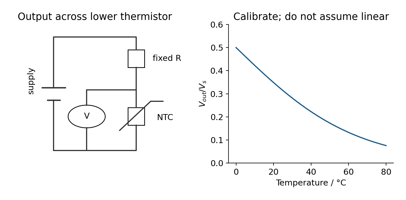
تحليل مقسّمات الجهد ذات المقاومة المتغيرة، بما في ذلك الثرمستورات ومكافئات الضوء.
تعريف القوة الدافعة الكهربائية والمقاومة الداخلية؛ التمييز بين القوة الدافعة الكهربائية وفارق الجهد الطرفي.
الممارسة العملية الأساسية 8: تحديد القوة الدافعة الكهربائية والمقاومة الداخلية لخلية كهربائية.
نمذجة مقاومة تعتمد على درجة الحرارة باستخدام اهتزازات الشبكة وعدد الإلكترونات الموصلة؛ تطبيق ذلك على المعادن والثرمستورات ذات معامل درجة الحرارة السالب.
نمذجة مقاومة تعتمد على الإضاءة باستخدام عدد الإلكترونات الموصلة؛ تطبيق ذلك على مكافئات الضوء.
المصدر: منهج كامبريدج الدولي
ورقة عمل
من إشارة الهاتف إلى بطاريته
يستقبل هاتفك موجات ويستخدم الطاقة الكهربائية. تبدو مختلفة، لكن كليهما يعتمد على نقل الطاقة. الموجات تنقل الطاقة دون حمل المادة معها. الدائرة الكهربائية تنقل الطاقة عبر حركة الشحنة.
يشمل هذا المرجع WPH12 الموجات والكهرباء، وبيانات المواصفة 33–80. مدة الامتحان 90 دقيقة ودرجته 80. استخدم قائمة الصيغ لدعم استنتاجاتك. اشرح لماذا يناسب معادلة الموقف، وأظهر التحويلات، وانهِ المقارنات بخلاصة.
كميات الموجات والرسوم البيانية
مصدر اهتزازي يعيد حركته. السعة هي أقصى إزاحة عن موضع الاتزان. الاتزان يعني وضع الراحة. الزمن الدوري$T$ هو الوقت لاهتزاز كامل واحد. التردد$f$ هو عدد الاهتزازات الكاملة كل ثانية؛ وحدته الهرتز، Hz.
$$f = \frac{1}{T} \qquad v = f\lambda$$
الطول الموجي$\lambda$ هو المسافة بين أقرب نقطتين تهتزتان في طور واحد. سرعة الموجة$v$ هي السرعة التي ينتقل بها طور ثابت، مثل القمة. وهي ليست سرعة جسيم مهتز.
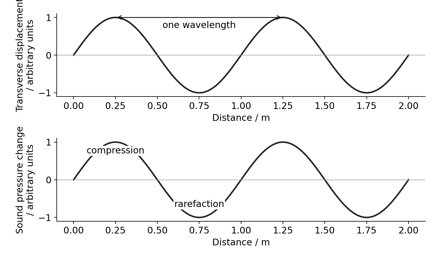
الموجة المستعرضة تكون اهتزازاتها عمودية على اتجاه انتشارها. الحبل يتحرك للأعلى والأسفل بينما تنتشر الاضطراب على طول الحبل.
الموجة الطولية تكون اهتزازاتها موازية لاتجاه انتشارها. الصوت يحتوي على تكثفات، حيث الضغط والكثافة أعلى، وتمددات، حيث تكون أقل.
تتحرك جزيئات الهواء ذهابًا وإيابًا حول مواقع راحتها. لا تسافر من مكبر الصوت إلى أذنك مع الصوت.
تُظهر الرسوم البيانية للمسافة موجة كاملة في لحظة واحدة.
اقرأ المحور الأفقي أولاً
مخطط الإزاحة–المسافة هو لقطة. مسافة الفصل بين قممتين متجاورتين تعطي $\lambda$. مخطط الإزاحة–الزمن يتتبع جسيمًا واحدًا. مسافة الفصل بين قمم متجاورة تعطي $T$. يمكن أن تمثل نفس شكل المنحنى كلا الرسمين، لكن الكميات مختلفة.
بالنسبة للموجة الطولية، يُظهر الرسم البياني للضغط-المسافة مناطق التضاغط عند ذروة الضغط. بينما يُظهر الرسم البياني لإزاحة الجزيئات-المسافة الإزاحة على طول اتجاه الانتشار. يحدث أقصى تضاغط حيث تتغير الإزاحة بسرعة نحو الجزيئات المجاورة. لا يقع الحد الأقصى للضغط والحد الأقصى للإزاحة في نفس المكان؛ وتكون أنماطهما متباعدة بربع طول موجي في موجة صوتية جارية ذات شكل جيبي.
مثال محلول. يسجل ميكروفون 12 دورة كاملة في $0.030\ \text{s}$. ينتقل الصوت بسرعة $340\ \text{m s}^{-1}$. أوجد تردده وطول موجته.
المعطيات: عدد الدورات، الوقت الكلي، والسرعة. التردد يحسب عدد الدورات في الثانية؛ ثم تربط معادلة الموجة السرعة بالطول الموجي.
الجبهة الموجية تجمع نقاطاً لها نفس الطور. يصف الطور مرحلة دورة الاهتزاز. تقابل دورة واحدة كاملة $360^\circ$ أو $2\pi$ راديان.
يعني التراكب جمع إزاحات الموجات المتداخلة عند كل نقطة. التداخل هو التعزيز الناتج أو الإلغاء. المصادر المتماسكة لها نفس التردد وفرق طور ثابت. قد لا يكون فرق الطور صفراً.
بالنسبة لموجات بنفس الطول الموجي، فإن فرق الطور الناجم عن فرق المسار$\Delta x$ هو:
بالنسبة للمصادر التي تبدأ بتوافق الطور، تعطي فروق المسار $0,\lambda,2\lambda,\ldots$ تداخلاً بنّاءً. أما فروق نصف طول موجة فتعطي تداخلاً هادماً. تتطلب الإلغاء الكامل أيضاً تساوي السعات. إذا كانت المصادر تبدأ بفارق طور، فأدرج ذلك أيضاً.
مثال محلول. نتجت مكبران صوتيان متشابهان الطور طول موجي $0.80\ \text{m}$. اختلفت مساراتهما نحو ميكروفون بمقدار $1.20\ \text{m}$.
المعطيات: فرق المسار والطول الموجي. حول فرق المسار إلى دورات، ثم إلى طور.
$540^\circ$ يعادل $180^\circ$. تصل الموجات بعكس الطرود وتتداخل تداخلاً هادماً. لا يجب أن يصبح الصوت صامتاً بالضرورة إذا اختلفت السعات الواردة.
كيفية تكون الموجة الموقوفة
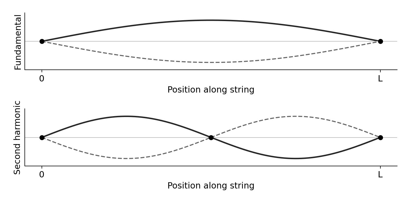
تتكون الموجة الموقوفة عندما تنتشر موجتان لهما نفس التردد وسعة مماثلة في اتجاهين متعاكسين وتترابطان. يوفر الانعكاس عند نهاية حبل ثابت الموجة العائدة.
دائماً ما يكون للعقدة (النقطة الصامتة) إزاحة صفرية. وللمنتصف عقدي (النقطة الحركية) أكبر سعة اهتزاز.
العقد المتجاورة تبعد عن بعضها $\lambda/2$. تبعد العقدة وأقرب منتصف عقدي عنها $\lambda/4$.
تهتز النقاط بين نفس الزوج من العقد بنفس الطور. تهتز النقاط في الأقسام المجاورة بعكس الطور.
جميع النقاط لها نفس التردد، باستثناء أن العقدة لا تهتز. تعتمد السعة على الموقع.
الموجة الموقوفة المثالية لا تنقل طاقة صافية عبرها. تحمل الموجة الجارية الطاقة على طول اتجاه انتشارها.
تبقى العقد النهائية ثابتة؛ ويتغير الشكل بين الخط المتصل والمنقط.
بالنسبة لوتر مثبت من الطرفين، يحتوي الطول $L$ على عدد صحيح $k$ من أنصاف الأطوال الموجية:
$$L = \frac{k\lambda}{2} \qquad v = \sqrt{\frac{T}{\mu}} \qquad f = \frac{k}{2L}\sqrt{\frac{T}{\mu}}$$
هنا $T$ هو الشد، وليس الدور؛ و$\mu$ هو الكتلة لكل وحدة طول بوحدة $\text{kg m}^{-1}$. التردد الأساسي يحتوي على $k=1$. عند وضع حد ثابت، يزداد التردد مع $\sqrt{T}$، وينقص مع $L$، وينقص مع $\sqrt{\mu}$.
مضاعفة الشد تضاعف التردد بمقدار $\sqrt{2}$، وليس الضعف الكامل.
صوت واقف في أنبوب مغلق
في أبسط موجات صوتية واقفة في أنبوب مغلق من طرف واحد، يكون الطرف المغلق عقدة إزاحة جزيئية. والطرف المفتوح تقريباً عقبة إزاحة. هذا يتوافق مع ربع طول موجي داخل الطول الفعال للأنبوب، لذا $L_{effective}=\lambda/4$. نمط الضغط معكوس: الطرف المغلق هو عقبة ضغط. لا تسمّ عقدة ضغط بعقدة إزاحة. الأنابيب الحقيقية لها تصحيح صغير للطرف المفتوح؛ استخدم الطول الفعال إذا زوّدت به المسألة.
مثال محلول. أنبوب مغلق طوله الفعال $0.20\ \text{m}$ وتردده الأساسي $425\ \text{Hz}$. تعطي شروط الأطراف $\lambda=4L=0.80\ \text{m}$؛ ثم $v=f\lambda=425\times0.80=340\ \text{m s}^{-1}$. بينما يتناسب الوتر المثبت من الطرفين مع نصف طول موجي في وضعه الأساسي. اختر من شروط الأطراف، وليس من كلمة "واقف".
عملي أساسي 4: سرعة الصوت
استخدم مولد إشارات، مكبر صوت، ميكروفون متحرك وراسم ذرات ثنائي الشعاع. وصّل قناة راسم الذرات الواحدة بإشارة المرجع للمولد والأخرى بمخرج الميكروفون. كلا المسارين لهما نفس التردد.
حافظ على التردد ثابتاً. حرك الميكروفون على خط مقاس مبتعداً عن مكبر الصوت. ابحث عن موقع تكون فيه المسارات في طور واحد.
انتقل إلى موقع آخر في طور واحد. مواقع الطور الواحد المتتالية تبعد مسافة طول موجي واحد. قِس عبر عدة أطوال موجية وقسّم على عددها.
اقرأ الدور من مقياس قاعدة الوقت: عد الوحدات الأفقية عبر عدة دورات، ثم قسّم. أوجد $f=1/T$ واستخدم $v=f\lambda$.
كرر المواقع والترددات. حافظ على الميكروفون على محور مكبر الصوت. قلل الصوت المنعكس بالعمل بعيداً عن الجدران. قِس الموقع من نقطة مرجعية ثابتة للميكروفون.
قياس عدة أطوال موجية يقلل عدم اليقين النسبي في المسافة. وقياس عدة دورات يفعل نفس الشيء للزمن. يمكن لتجربة الأنبوب الرنان أيضاً قياس سرعة الصوت، لكنها لا تحل محل العملي المحدد هذا.
عملي أساسي 5: وتر اهتزازي
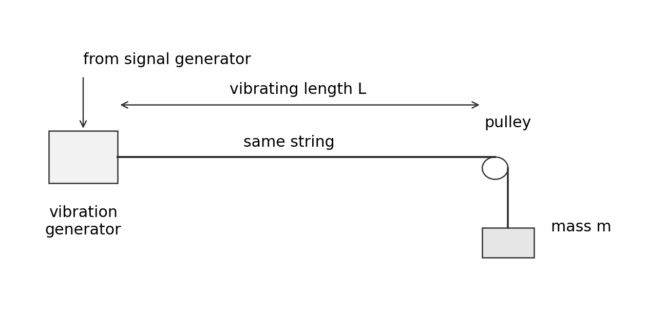
استخدم مولد اهتزازات يُشغّل بواسطة مولد إشارات. مرر الوتر فوق عجلة نحو كتلة معلّقة. يكون الشد حوالي $mg$ عندما تكون احتكاك العجلة ضئيلاً. زد التردد حتى تتشكل نمط موجة واقفة واضح.
تحقيق الشد: احفظ $L$، $\mu$ والوضع ثابتين. غيّر الكتلة المعلّقة. ارسم $f^2$ مقابل $T$؛ ميل المنحنى للتردد الأساسي هو $1/(4L^2\mu)$.
تحقيق الطول: احفظ الشد ونوع الوتر والوضع ثابتين. ارسم $f$ مقابل $1/L$.
استقصاء الكثافة الخطية: قِس كتلة الخيط وطوله، $\mu=m/l$. استخدم خيوطاً مختلفة بتوتر ثابت وطول اهتزاز ونمط محدد. ارسم $f^2$ مقابل $1/\mu$.
قِس الطول بين العقد الطرفية. حدد التوافق من ترددات أعلى وأقل وأعد القياس. ثبت الحامل وابتعد عن الأثقال الساقطة.
الشدة والانكسار والاستقطاب
الشدة هي القدرة لكل وحدة مساحة عمودية على اتجاه تدفق الطاقة:
$$I = \frac{P}{A}$$
وحدة قياسها هي $\text{W m}^{-2}$. بالنسبة للمستقبل، تكون القدرة الساقطة $P=IA$. يكون المخرجات المفيدة أقل إذا كانت الكفاءة أقل من 100%. حول المساحة بعناية: $1\ \text{cm}^2=10^{-4}\ \text{m}^2$.
مثال محلول. شدة الإشعاع تساوي $800\ \text{W m}^{-2}$ على خلية شمسية مساحتها $25\ \text{cm}^2$. الكفاءة هي 20%. هل يمكنها تزويد $0.50\ \text{W}$؟
المعطيات: الشدة، المساحة، الكفاءة. أولاً احسب القدرة الساقطة، ثم القدرة المفيدة.
$0.40\ \text{W}<0.50\ \text{W}$، لذا لا يمكنها تزويد القدرة المفيدة المطلوبة.
الانكسار والانعكاس الكلي الداخلي
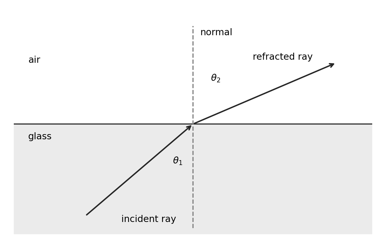
الانكسار هو تغير في اتجاه الموجة عند تغير سرعتها عند الواجهة. الشعاع الذي يدخل على طول العمود يتغير سرعته دون أن يتغير اتجاهه. العمود هو الخط العمودي على الحدود. قِس جميع زوايا الشعاع بدءاً منه.
معامل الانكسار$n$ يقارن سرعة الضوء في الفراغ $c$ مع سرعتها في المادة. يبقى التردد ثابتاً عبر الحدود، لذا يتغير الطول الموجي مع السرعة. الدخول في معامل انكسار أعلى $n$ يُقوّع الشعاع نحو العمود؛ والدخول في معامل أقل $n$ يُقوّعه بعيداً عنه.
ينحرف الشعاع بعيداً عن العمود عندما يدخل في الوسط ذي معامل الانكسار الأقل.
يتطلب الانعكاس الكلي الداخلي الانتقال من وسط ذات معامل انكسار أعلى إلى آخر أقل وزاوية سقوط أكبر من الزاوية الحرجة$C$.
$$\sin C = \frac{n_2}{n_1} \qquad \text{for material to air: }\sin C = \frac{1}{n}$$
عند $C$ تكون زاوية الانكسار $90^\circ$؛ نسمي السقوط الأكبر من $C$ انعكاساً كلياً داخلياً. أسفل $C$، تنعكس عادةً بعض الطاقة وتنتقل أخرى. تستخدم الألياف الضوئية قلباً ذو معامل انكسار أعلى وغلافاً أقل. رفع معامل انكسار الغلاف يرفع الزاوية الحرجة ويمكن أن يمنع شعاعاً كان منعكساً سابقاً من البقاء محبساً.
مثال محلول. يسير الضوء من زجاج معامل انكساره 1.50 إلى الهواء. هل ينتج زاوية سقوط مقدارها $45^\circ$ انعكاساً كلياً داخلياً؟
المعطيات: المعاملاان وزاوية السقوط. أوجد زاوية الحدود قبل المقارنة.
يسير الضوء نحو معامل انكسار أقل و$45^\circ>41.8^\circ$. تتحقق الشرطان معاً، فيحدث انعكاس كلي داخلي.
قياس معامل الانكسار
ضع مكعباً شفافاً مستطيل الشكل على ورقة ورسم حدوده. استخدم حزمة ضيقة من صندوق أشعة. عيّن نقطتين على الشعاع الساقط ونقطتين على الشعاع الخارج. أزل المكعب وصِل نقاط الحدود لإعادة بناء الشعاع داخله. ارسم العمود عند الدخول وقيِّس زاوية السقوط $i$ وانكساره $r$ باستخدام المنقلة.
كرر لعدة زوايا سقوط، مع الحفاظ على نفس المادة ولون الضوء. ارسم $\sin i$ عموديًا مقابل $\sin r$ أفقيًا. بالنسبة للضوء المار من الهواء إلى المكعب، يمثل الميل معامل انكسار المكعب نسبيًا للهواء. استخدم مثلثًا كبيرًا على خط أفضل ملاءمة. الحزم الضيقة وعلامات الأشعة المتباعدة تقلل من عدم اليقين في الاتجاه. الزوايا الصغيرة جدًا تعطي نسبة خطأ زاوية كبيرة.
الاستقطاب المستوي
الاستقطاب المستوي يقيص الاهتزازات العرضية في مستوى واحد يحتوي على اتجاه الانتشار. ضوء غير مستقطب له اهتزازات في مستويات متعددة. يقوم المستقطب بنقل اتجاه اهتزاز واحد. قم بتدوير مستقطب ثانٍ: التوازي في اتجاهات النقل يعطي أقصى سطوع؛ التعامد يعطي ظلامًا مثاليًا. ما يزال الشعاع يتقدم للأمام؛ تتغير اتجاهات اهتزازه بالاختيار.
الموجات الطولية لا يمكن استقطابها مستويًا لأن اهتزازها يكون بالفعل على طول الانتشار. لذلك، يُعد الاستقطاب دليلاً على أن الضوء موجة عرضية.
الحيود ونبضة الصدى
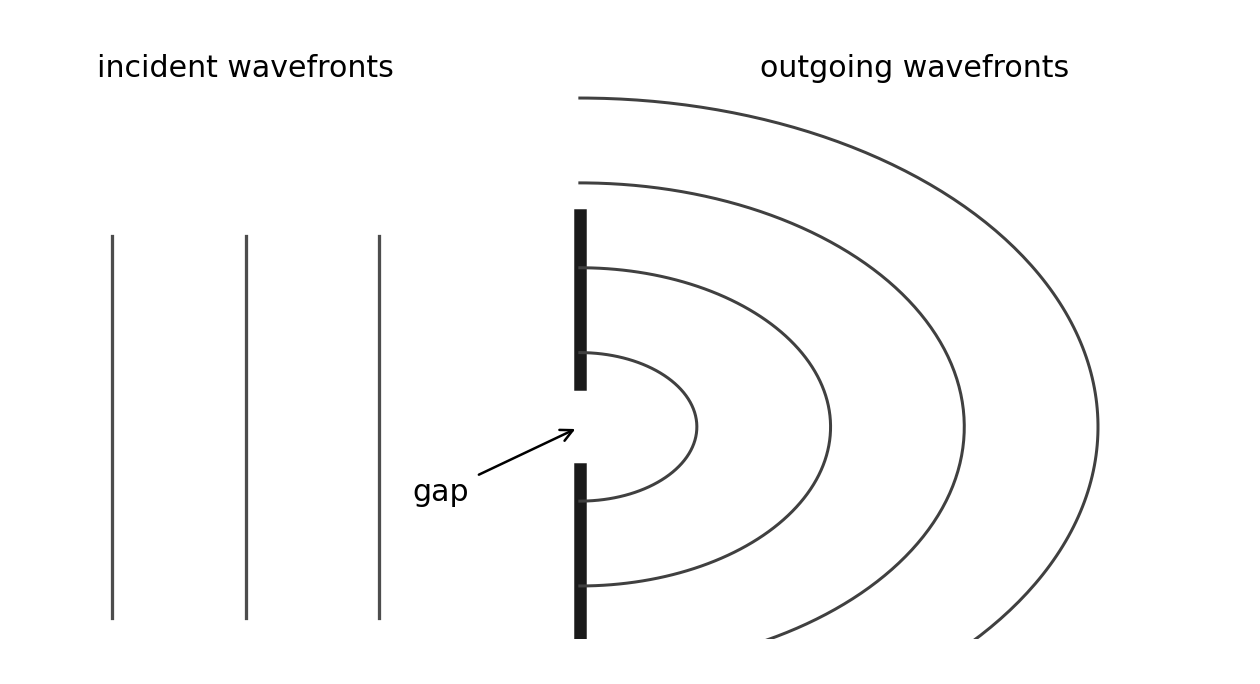
الحيود هو انتشار الموجات عند فتحة أو حافة. يكون الانتشار أكبر عندما تكون عرض الفتحةComparable لطول الموجة. لا تزال الفتحة الواسعة يحدث فيها حيود عند حوافها، لكن الموجة المركزية تنتشر أقل.
في بناء هيجنس، تعمل كل نقطة على جبهة الموجة كمصدر لموجات ثانوية. ارسم موجات ثانوية بنفس نصف القطر بعد نفس الوقت. يعطي مماسها المشترك الأمامي الجبهة الموجية الجديدة. عند فتحة ضيقة،只提供 جزء صغير فقط من الجبهة الأصلية موجات ثانوية، لذا تنتشر الجبهات emerging على نطاق واسع. هذا يفسر الانتشار دون افتراض تغيير في التردد عند الشق.
الفتحة تحدد أي النقاط توفر الموجات الثانوية الخارجة.
شبكات الحيود والممارسة الأساسية 6
شبكة الحيود تحتوي على عدد كبير من الشقوق متساوية المسافة. تظهر الحد الأقصى الساطع عندما تصل مساهمات من شقوق مجاورة في طور:
$$k\lambda = d\sin\theta$$
هنا $k$ هو العدد الصحيح الرتبة، $d$ هو تباعد الشقوق، و$\theta$ مقاسة من الاتجاه المستقيم. تفترض المعادلة السقوط العمودي. إذا كانت الشبكة تحتوي على $N$ خطوط لكل متر، فإن $d=1/N$. لا تخلط بين رتبة الشبكة ومعامل الانكسار؛ قد تستخدم الأوراق المطبوعة $n$ لكلاهما.
مثال محلول. شبكة تحتوي على 600 خطوط لكل مليمتر. يظهر ضوء الرتبة الأولى عند $18.0^\circ$. أوجد طوله الموجي.
معلوم: كثافة الخط وزاوية الرتبة الأولى. حول كثافة الخط قبل أخذ مقلوبه.
هذا هو $515\ \text{nm}$. تحقق من كل رتبة أعلى مقترحة باستخدام $k\lambda/d\leq1$.
بالنسبة لتجربة CP6، وجه ليزر منخفض القدرة عموديًا على الشبكة وضع شاشة عمودية على الشعاع المركزي. قِس مسافة الشاشة $D$ والإزاحة $x$ من البقعة المركزية إلى رتبة معينة. استخدم $\tan\theta=x/D$، ثم معادلة الشبكة. اجمع الإزاحات المقابلة يسارًا/يمينًا، كرر القياسات، واستخدم الرتب المرئية الأعلى حيث القياس واضح. قِس من الشبكة إلى الشاشة، وليس من غلاف الليزر. لا تعوّض $\sin\theta=x/D$ إلا إذا كان تقريب الزاوية الصغيرة المبرر مقبولاً. لا تنظر أبدًا داخل الشعاع؛ احتفظ به أسفل مستوى العين وأوقف الأشعة المشتتة.
الإلكترونات تُظهر أيضًا سلوكًا موجيًا
حزمة إلكترونات تمر عبر بلورة رقيقة تنتج نمط حيود. يوفر تباعد الذرات المنتظم بنية الحيود. تغيير زخم الإلكترون يغير تباعد النمط. هذا دليل على السلوك الموجي؛ لا يمكن للجسيمات التي تسافر على مسارات مستقيمة بسيطة وحدها تفسير حدائق الحيود القصوى.
الطول الموجي دي برولي هو:
$$\lambda = \frac{h}{p}$$
بالنسبة لإلكترون غير نسبي، $p=mv$. إذا اكتسب طاقة حركية عن طريق عبور فرق جهد، فإن $E_k=eV$ و$p=\sqrt{2mE_k}$. استخدم هذه الروابط فقط عندما تعطيك السؤال أو تتطلب تلك العلاقة للطاقة.
مثال محلول. يمتلك إلكترون زخم $2.0\times10^{-24}\ \text{kg m s}^{-1}$. مع $h=6.63\times10^{-34}\ \text{J s}$:
زيادة الزخم تقلل الطول الموجي. للإلكترونات خصائص جسيمية وموجية؛ لا يعني الانتشار أن الإلكترون يتحول إلى موجة صوتية.
الانعكاس والنقل والصدى
عند الواجهة، قد يُنتَجز جزء من طاقة الموجة وينعكس جزء آخر. يمكن للمنبعث المنعكس تحديد الحدود. في الصدى النبضي، يشمل التأخير المقاس الرحلة ذهاباً وإياباً:
$$2s = vt \quad\Rightarrow\quad s = \frac{vt}{2}$$
مثال محلول. ينتشر الصوت فوق الصوتي في المعدن بسرعة $5900\ \text{m s}^{-1}$. يعود صدى بعد زمن $12\ \mu\text{s}$.
تقع الحدود على مسافة $35\ \text{mm}$، وليس $71\ \text{mm}$. قد يتداخل الصدى القريب مع المنبثع المُرسَل. يقلل قصر مدة النبض هذه المنطقة العمياء ويفصل بين الأصداء المتقاربة. يساعد الطول الموجي القصير في اكتشاف أو التمييز بين الميزات الأصغر. هذه حدود مترابطة، لكن مدة النبض والطول الموجي ليسا نفس الكمية. استخدم السرعة في المادة الفعلية، وليس تلقائياً سرعة الهواء.
الفوتونات والتأثير الكهروضوئي
تُفسر أفكار الموجات التداخل والانتشار والاستقطاب. لم تفسر جميع ملاحظات انتقال الطاقة. تصف الفوتونات حزماً منفصلة من الطاقة الكهرومغناطيسية:
$$E = hf = \frac{hc}{\lambda}$$
تاريخياً، دعم التداخل والانتشار نماذج الموجات للضوء. تطورت الأفكار الكمية لتفسير مشاهدات بما فيها التأثير الكهروضوئي وأطياف الذرة. تستخدم الفيزياء الحديثة كلا الوصفين الموجي والفوتوني وفقاً للقياس. يجب أن يفسر النموذج الجديد الناجح الأدلة التي يفسرها النموذج القديم أيضاً.
فوتون واحد وإلكترون واحد
في التأثير الكهروضوئي، يمتص إلكترون السطح فوتوناً وقد يهرب. دالة الشغل$\phi$ هي الحد الأدنى للطاقة اللازمة لإزالة إلكترون من السطح. تردد العتبة هو $f_0=\phi/h$.
تحت العتبة، لا يسبب زيادة الشدة انبعاثاً في نموذج الفوتون الفردي المعتاد.
فوق العتبة، raises تردد أعلى الطاقة الحركية القصوى. بيانه البياني لـ $E_{k,\max}$ مقابل $f$ له ميل $h$، وقاطع التردد $f_0$ وقاطع الطاقة المستخرج $-\phi$.
عند ثبات التردد فوق العتبة، توفر شدة أعلى فوتونات أكثر في الثانية. يمكن إطلاق إلكترونات أكثر في الثانية، لذا يرتفع تيار الضوء المشبع. لا ترتفع طاقتها الحركية القصوى.
يبدأ الانبعاث بدون تأخير بناء الطاقة المتوقع من نموذج الطاقة الموجية المستمرة البسيط، حتى عند الشدة المنخفضة فوق العتبة.
تهرب الإلكترونات بطاقة حركية متنوعة. تفقد البعض طاقة أكبر داخل المادة. المعادلة تصف الطاقة العظمى، ليست طاقة كل إلكترون.
الإلكترون فولت وحدة طاقة: $1\ \text{eV}=1.60\times10^{-19}\ \text{J}$. إنها ليست وحدة فرق جهد. جهد الإيقاف $V_s$ يمنع فقط الوصول إلى المجمع لأكثر إلكترونات ضوئية سرعة، لذا $eV_s=E_{k,\max}$.
مثال محلول. يصل ضوء بتردد $8.0\times10^{14}\ \text{Hz}$ إلى سطح لدالة شغل $2.0\ \text{eV}$.
معلوم: تردد الفوتون ودالة الشغل. حول دالة الشغل إلى جول قبل طرحها.
تؤكد الطاقة الحركية الإيجابية أن هذا التردد فوق العتبة. يعني الطرح السلبي عدم وجود انبعاث، وليس طاقة حركية سالبة.
الأطياف الخطية الذرية
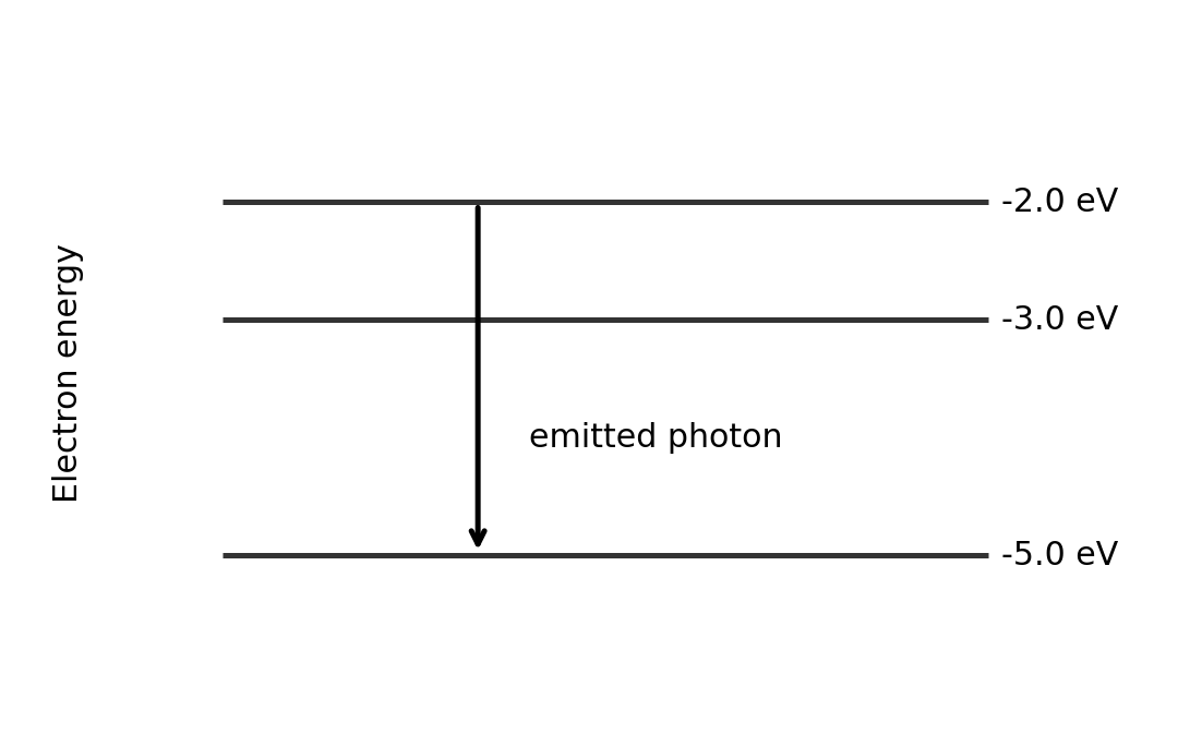
تتمتع الذرات بـ مستويات طاقة منفصلة. عند انتقال الإلكترون من مستوى مسموح إلى آخر أدنى، يُصدر فوتوناً. أما الانتقال لأعلى فيمتص الطاقة المماثلة:
$$|\Delta E| = hf = \frac{hc}{\lambda}$$
يتميز الطيف الخطي بتواترات محددة لأن فروق المستويات المسموحة محدودة. أكبر فرق طاقى هبوطياً يعطي أعلى تواتر وأقصر طول موجي. احسب الانتقالات الممكنة بفحص أزواج المستويات والمستويات العليا المعبأة؛ لا تحسب عدد الخطوط مساوياً لعدد المستويات تلقائياً.
طاقة الفوتون تساوي الفرق بين المستويين.
مثال محلول. يسقط إلكترون من $-2.0\ \text{eV}$ إلى $-5.0\ \text{eV}$.
لا يؤدي امتصاص الضوء في المادة دائماً إلى إخراج إلكترون من سطحها. فعملية الإثارة متبوعة بالانبعاث، كما يحدث في المواد النشطة ضوئياً، ليست آلياً ظاهرة الكهروضوئية.
التيار والمقاومة والدوائر الكهربائية
التيار هو معدل تدفق الشحنة. يتبع التيار التقليدي الاتجاه الذي ستتحرك فيه الشحنات الموجبة. وفي المعدن، تتحرك الإلكترونات عكس هذا الاتجاه.
$$I = \frac{\Delta Q}{\Delta t} \qquad V = \frac{W}{Q} \qquad R = \frac{V}{I}$$
الأمبير الواحد هو كولوم واحد في الثانية. فرق الجهد$V$ هو الطاقة المنتقلة لكل وحدة شحنة بين نقطتين. المقاومة $R$ تُعرف من خلال النسبة $V/I$ عند نقطة تشغيل. قانون أوم هو الشرط الإضافي $I\propto V$ عندما تبقى درجة الحرارة والعوامل الفيزيائية الأخرى ثابتة. لا تطيع كل مقاومة أو مكون هذا القانون.
مثال محلول. يمر تيار قدره $0.40\ \text{A}$ لمدة $30\ \text{s}$. أوجد عدد الإلكترونات التي تمر بنقطة ما.
$$Q = It = 0.40\ \text{A}\times30\ \text{s} = 12\ \text{C}$$
للمجموعة المتصلة على التوازي مقاومة أصغر من أقل مقاومة في فروعها. يُوصل الفولتميتر على التوازي عبر المكون؛ والفولتميثر المثالي له مقاومة لا نهائية. يُوصل الأميتر على التوالي؛ والأميتر المثالي له مقاومة صفرية.
مثال محلول. مقاومة $6.0\ \Omega$ متصلة بالتوازي مع $3.0\ \Omega$. المجموعة متصلة على التوالي مع $4.0\ \Omega$ عبر مصدر جهد $12\ \text{V}$.
معلوم: ترتيب الدائرة. قلل قسم التوازي أولاً، ثم طبق قاعدة التوالي.
تحقق: تجمعات تيارات الفروع تساوي $2.0\ \text{A}$. توجد هبوطية قدرها $8.0\ \text{V}$ في المقاومة المتبقية المتصلة على التوالي.
القدرة ومخططات المكونات
الطاقة الكهربائية هي الطاقة المنقولة في كل ثانية. بتعويض $V=IR$ في $P=VI$ نحصل على الصيغ الأخرى:
$$P = VI = I^2R = \frac{V^2}{R} \qquad W = Pt = VIt$$
استخدم الجهد عبر المكون، والتيار المار فيه. تنطبق قوانين المقاومة على مقاومته عند نقطة التشغيل؛ لا تفترض أن مصباح التسخين له مقاومة ثابتة.
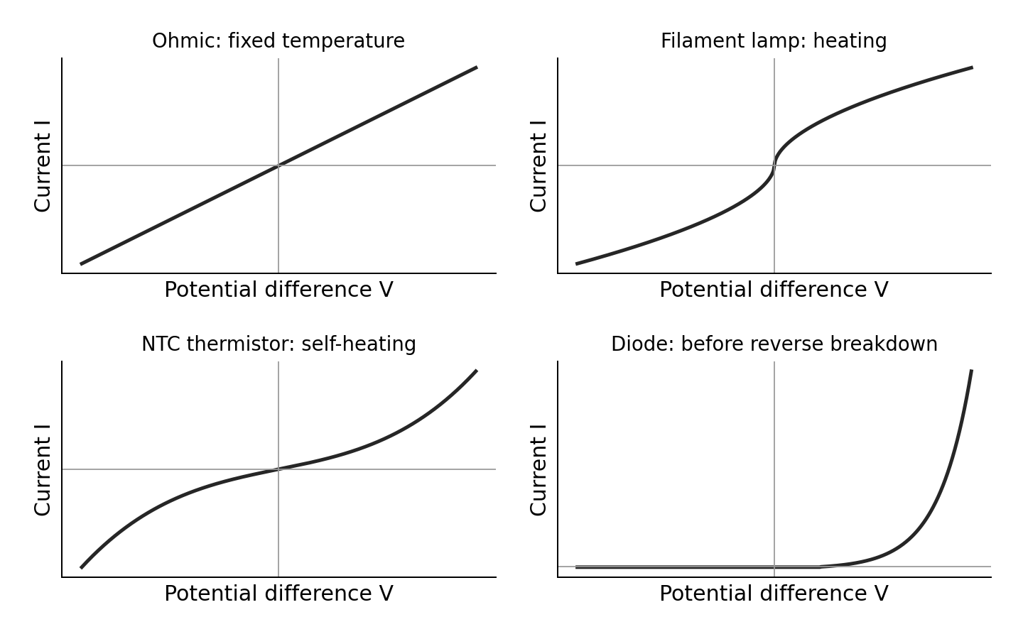
المحاور وشروط درجة الحرارة مهمة عند تفسير هذه المنحنيات التخطيطية.
موصل أومي عند درجة حرارة ثابتة: خط مستقيم يمر بالمبدأ. على رسم بياني يكون $I$ عموديًا و$V$ أفقيًا، يكون ميله $1/R$.
مصباح خيطي: مع زيادة مقدار الجهد، يزداد التسخين فتزيد المقاومة. يصبح منحنى $I$–$V$ أقل انحدارًا.
مقياس حراري NTC: يخفض التسخين المقاومة. إذا قوّى التيار تسخينه بشكل كافٍ، يصبح المنحنى أكثر انحدارًا. عند درجة حرارة ثابتة متحكم بها، يمكن أن يكون سلوكه خلال نطاق مناسب تقريبًا أوميًا. لا تدعي أن منحنيات كل مقاييس حرارية يجب أن تنحني تحت أي ظرف قياس.
الديود: تيار عكسي صغير جدًا قبل الانهيار؛ يتزايد التيار الأمامي بسرعة بعد ركن مميز. هو يوصل بشكل رئيسي في اتجاه واحد. الديود الحقيقي ليس له مقاومة واحدة ثابتة.
بالنسبة للرسم البياني المنحني، يستخدم $R=V/I$ خطًا من المبدأ إلى نقطة التشغيل. ميل المماس ليس عمومًا $1/R$.
المقاومة النوعية والتجربة الأساسية 7
المقاومة النوعية$\rho$ هي خاصية للمادة عند درجة حرارة محددة:
$$R = \frac{\rho l}{A} \qquad A = \frac{\pi d^2}{4}$$
زيادة طول سلك موحد تزيد المقاومة. زيادة مساحة المقطع العرضي تقللها. مضاعفة القطر تعطي أربعة أضعاف المساحة وربع المقاومة، إذا بقيت المادة والطول ودرجة الحرارة دون تغيير.
لتجربة CP7، قم بتوصيل سلك موحد، أميتر، مصدر طاقة، مفتاح ومقاومة لتقييد التيار على التوالي. وصل فولتميترًا عبر طول السلك المقاس. قس عدة أطوال وأوجد $R=V/I$ لكل منها. ارسم $R$ مقابل $l$: الميل $=\rho/A$، إذن $\rho=A\times\text{gradient}$.
قِس القطر بميكرومتر عند مواضع واتجاهات متعددة؛ تحقق من صفريته. قِس الطول بين نقاط الاتصال الكهربائية الفعلية. استخدم تيارًا صغيرًا وقفّ المفتاح بين القراءات لتقييد التسخين. حافظ على اتصالات contacts آمنة. قد يشير تقاطع غير صفري إلى مقاومة اتصال أو أسلاك. تكرار القراءات يقلل التشتت لكن لا يزيل خطأ صفر القطر. بما أن المساحة تعتمد على $d^2$، فإن عدم يقين طفيف بالمئوية في القطر يساهم بحوالي ضعف تلك المئوية في عدم يقين المساحة.
مثال محلول. قطر السلك هو $0.40\ \text{mm}$. الرسم البياني لـ$R$–$l$ له ميل $3.5\ \Omega\,\text{m}^{-1}$.
سرعة الانجراف$v$ هي متوسط السرعة الموجهة الصغيرة لحاملي الشحنة، وليست سرعتها الحرارية العشوائية:
$$I = nqvA$$
هنا $n$ هو عدد الحاملات المتحركة لكل وحدة حجم، $q$ هو مقدار شحنة كل حامل، و$A$ هو مساحة المقطع العرضي. الكثافة الأكبر للحاملات تسمح بنفس التيار بسرعة انجراف أقل. في الأسلاك المتصلة على التوالي يكون التيار متساويًا؛ تغيير $n$ أو $A$ يغير $v$.
للمواد مقاومات نوعية مختلفة بسبب اختلاف كثافات حاملاتها وسهولة حركة حواملها. يزيد التشتت من سرعة الانجراف لنفس التدرج الجهد المطبق. كثافة الحامل وحدها لا تفسر كل الاختلافات بين المواد.
مجزئات الجهد، المستشعرات والخلايا
على طول سلك موحد يحمل تيارًا مستمرًا عند درجة حرارة ثابتة، تزداد المقاومة تناسبًا طرديًا مع المسافة. وبالتالي تزداد الانخفاض في الجهد التناسب الطردي مع المسافة أيضًا. بياني الجهد-المسافة يكون خطًا مستقيمًا. يفترض هذا المادة الموحدة والمساحة؛ السلك المدبب أو غير المتساوي التسخين قد لا يعطي خطًا مستقيمًا.
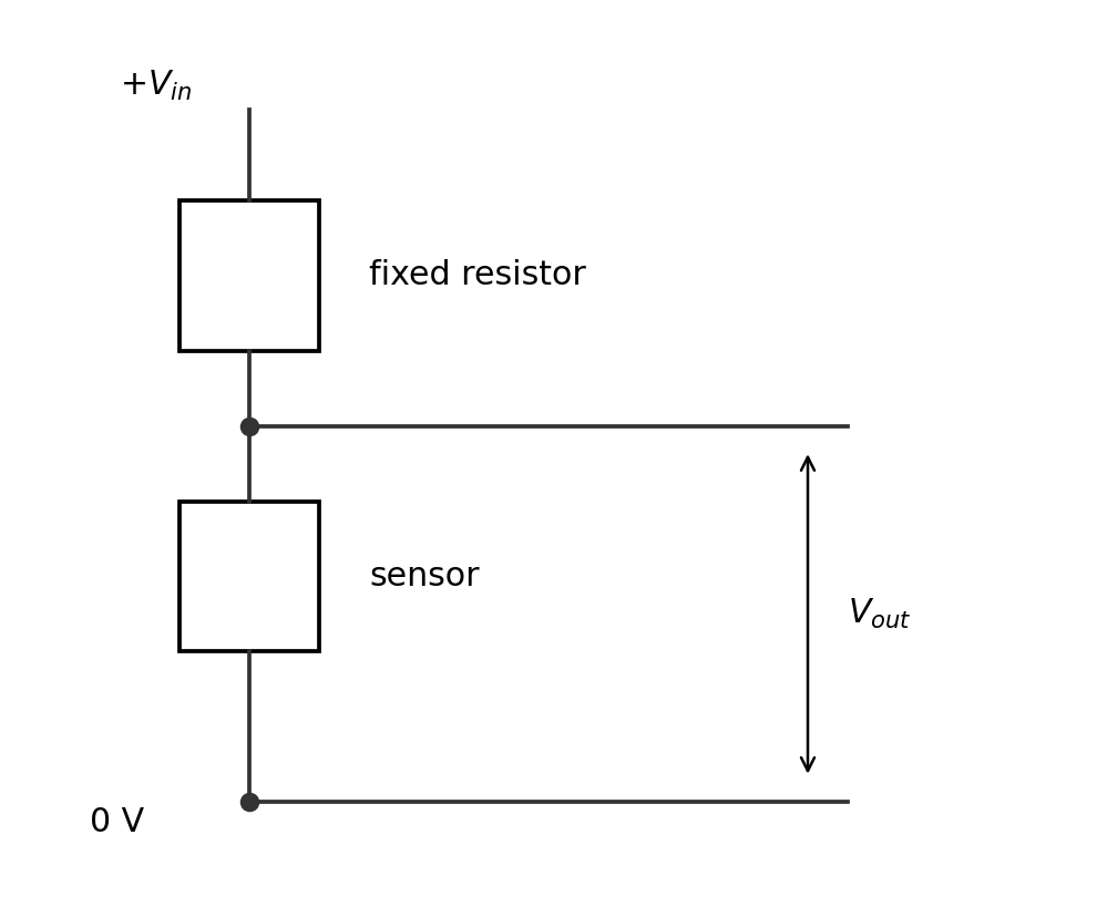
مقسِّم الجهد يستخدم مقاومات متسلسلة لتوزيع جهد المصدر:
يفترض التعبير أن الخرج غير محمول، أو أن الحمل المتصل يسحب تيارًا مهملاً. إذا سحب الحمل تيارًا كبيرًا، فاجمعها بالتوازي مع مقاومة الخرج أولاً. حدد دائمًا أي مقاومة يقيس عليها الفولتميتر.
تبديل الحساس والمقاومة الثابتة يعكس اتجاه تغير الخرج.
مثال محلل. مصدر $6.0\ \text{V}$ يغذي مقاومة ثابتة $2.0\ \text{k}\Omega$ فوق حساس ضوئي LDR. أوجد الخرج عبر LDR عندما تتغير مقاومته من $4.0$ إلى $1.0\ \text{k}\Omega$.
ينخفض الخرج عبر هذا LDR عند زيادة الإضاءة. يرتفع الخرج عبر المقاومة الثابتة. اشرح الخرج المسمى، وليس فقط “يتغير الجهد”.
شرح الحواسيس باستخدام حاملات الشحنة
في المعدن، يزيد التسخين اهتزازات الشبكة البلورية. تتشتت إلكترونات التوصيل بشكل متكرر. يبقى عدد الإلكترونات القابلة للحركة ثابتًا تقريبًا، لكن سرعة الانجراف عند تدرج جهد معين تقل، لذلك تزداد المقاومة.
في المقاومة الحرارية ذات معامل درجة الحرارة السالب، يحرر التسخين المزيد من حاملات الشحنة القابلة للحركة. يهيمن زيادة كثافة حاملات الشحنة، لذلك تقل المقاومة. تجنب قول إن التسخين يقلل اهتزازات الشبكة.
في المقاومة الضوئية (LDR)، يحرر الضوء الممتص حاملات شحنة إضافية قابلة للحركة. تزيد الإضاءة من كثافة حاملات الشحنة وتقلل المقاومة. لا يشترط أن تعمل بإلكترونات مغادرة سطحه.
للشرح المرتبط، قدم السلسلة الكاملة: تغيير بيئي → تغيير في حامل/تشتت → تغيير في المقاومة → تغيير في كسر المقسم → تغيير في الخرج المسمى. احتفظ بترتيب الدائرة في الاعتبار طوال الوقت.
القوة الدافعة الكهربائية، المقاومة الداخلية والتطبيق العملي 8
القوة الدافعة الكهربائية$\mathcal{E}$ هي الطاقة التي يوفرها المصدر لكل وحدة شحنة. تقاس بالفولت، على الرغم من اسمها. المقاومة الداخلية$r$ تسبب نقل الطاقة داخل المصدر عند مرور التيار. فرق الجهد الطرفي هو الطاقة لكل كولوم المتاحة للدائرة الخارجية:
$$\mathcal{E} = V+Ir \qquad V = \mathcal{E}-Ir \qquad I = \frac{\mathcal{E}}{R+r}$$
يوفر المصدر قدرة $\mathcal{E}I$، تستقبل الدائرة الخارجية $VI$، والاحتواء الداخلي هو $I^2r$. هذه تُجمع بشكل متسق. مع تيار مهمل، يقترب فرق الجهد الطرفي من القوة الدافعة الكهربائية.
لتطبيق عملي CP8، وصّل خلية، أميتر، حمل متغير ومفتاح على التوالي. وصّل فولتميتر عالي المقاومة عبر طرفي الخلية. غيّر المقاومة الخارجية وسجل أزواجًا من $V$ و$I$. ارسم $V$ عموديًا مقابل $I$ أفقيًا. الخط الأفضل مطابقة له له تقاطع $\mathcal{E}$ وميل $-r$. خذ مقدار الميل لـ $r$.
استخدم عدة إعدادات وأعد. افتح المفتاح بين القراءات، وتجنب مقاومة الحمل الصغيرة جدًا، واحافظ على درجة حرارة الخلية وحالتها المشحونة ثابتة قدر الإمكان. لا تقم أبدًا بتدوير الخلية. الرسم البياني المنحني قد يشير إلى تغير المقاومة الداخلية أو القوة الدافعة الكهربائية؛ لا تجبر خطًا واحدًا ثابتًا $r$ عليه دون مناقشة القيد.
مثال محلل. يمر رسم بياني للخلية عبر $(0.20\ \text{A},1.40\ \text{V})$ و$(0.60\ \text{A},1.20\ \text{V})$.
معلوم: نقطتان على الخط الأفضل مطابقة. ميل $V=\mathcal{E}-Ir$ هو $-r$.
تحقق باستخدام النقطة الثانية: $1.20+0.60\times0.50=1.50\ \text{V}$ أيضًا. ينخفض فرق الجهد الطرفي مع ارتفاع التيار.
تحقق من نفسك
استخدم ورقة التمرين الموصولة بعد كل قسم: 2.1 منحنيات الموجات؛ 2.2 الموجات الراكدة؛ 2.3 الانكسار؛ 2.4 الانحراف؛ 2.5 الفوتونات؛ 2.6 الدوائر الكهربائية؛ 2.7 مقسمات الجهد والخلية.
قبل استخدام مجموعة من الامتحانات السابقة، تحقق مما يلي:
قراءة المحاور وتحديد ما إذا كانت تعطي الطول الموجي، أو الدور، أو الضغط، أو الإزاحة؛
شرح تجربة عملية مع Apparatus (معدات)، وقياسات، ومتغيرات مسيطرة، ومنحنى بياني، وإجراءات احترازية؛
التمييز بين الطور والسعة، وتردد الفوتون ومعدل وصول الفوتونات؛
استنتاج تركيبات الدوائر الكهربائية من قانوني حفظ الشحنة والطاقة؛
شرح دائرة الحساس كمسبب مترابط سببيًا؛
استخدام مقارنة فعلية لإنهاء "استنتج ما إذا"، مع الوحدات واستنتاج واضح.
توفر الامتحانات 2025 لشهرَي يناير ويونيو أمثلة حقيقية، لكنها لا تختبر جميع المتطلبات. يملأ التدريب الأصلي الفجوات التعليمية. إكمال نموذج امتحان عينة وحده لا يثبت تغطية المنهج بالكامل.
Pearson Edexcel IAL Physics Issue 3 (يوليو 2021)، مطبوع ص24–ص26 والإلحاق 10 ص75–ص77. هذه تقسيمات تعليمية محلية، وليست عبارات محددة رسمية مرقمة.
تخطيط تجربة: اختيار المعدات ونطاق/دقة الأداة المناسبة؛ مناقشة المعايرة وفحص الصفر؛ وصف التقنيات الصحيحة للقياس؛ تحديد والتحكم في المتغيرات الأخرى ذات الصلة؛ الحكم على مدى مناسبة القراءات المتكررة؛ تحديد قضايا الصحة والسلامة والتدابير العملية؛ شرح معالجة البيانات؛ تحديد عدم اليقين/الأخطاء المنهجية وطرق تقليلها أو إزالتها؛ مناقشة فوائد/مخاطر وسياق اجتماعي أو بيئي أو تاريخي.
المصدر: منهج كامبريدج الدولي
3.2القياس والتسجيل وعدم اليقين
Pearson Edexcel IAL Physics Issue 3 (يوليو 2021)، مطبوع ص24–ص26 والإلحاق 10 ص75–ص77. هذه تقسيمات تعليمية محلية، وليست عبارات محددة رسمية مرقمة.
التنفيذ والقياسات: تقييم عدد ونطاق القراءات؛ تسجيل الأرقام الهامة بشكل متسق مع الدقة؛ فحص القراءات غير المتسقة بدلاً من حذفها بصمت؛ قراءة الأدوات، بما في ذلك الكاليبر الشفافي (0.1 مم) والميكرومتر (0.01 مم)؛ اقتراح معدات إضافية أو تقنيات محددة لتحسين القياس. تحديد عدم الي百分比 للقراءة الواحدة باستخدام نصف دقة الأداة، وعدم اليقين للقراءات المتكررة باستخدام نصف النطاق. تطبيق معاني الإلحاق 10 للدقة، والدقة، والتكرارية، والقابلية للتكرار، والصحة، والخطأ، وعدم اليقين، والدقة.
المصدر: منهج كامبريدج الدولي
3.3الرسوم البيانية، المعالجة والاستنتاجات المبررة
Pearson Edexcel IAL Physics Issue 3 (يوليو 2021)، مطبوع ص24–ص26 والإلحاق 10 ص75–ص77. هذه تقسيمات تعليمية محلية، وليست عبارات محددة رسمية مرقمة.
معالجة النتائج: الحساب بالأرقام الهامة المناسبة والوحدات؛ اختيار محاور/مقاييس الرسم البياني ورسم البيانات؛ تفسير العلاقة واستنتاج ثابت من الرسم البياني باستخدام مثلث ميل كبير; اقتراح تحسينات واقعية; مناقشة عدم اليقين نوعياً/كمياً; مقارنة فترة مقاسة مع قيمة مقترحة/معتمدة. لا تتطلب الوحدة 3 ضرب عدم اليقين المئوي. حدد نطاقاً مناسباً وبيانات مستهدفة إضافية بالقرب من الحد الأقصى عندما يتطلب الطلب ذلك.
المصدر: منهج كامبريدج الدولي
ورقة عمل
الرقم يحتاج إلى طريقة
مجموعتان تقومان بقياس نفس السلك. تختلف قيمتهما. أيهما يجب أن تثق؟ تحتاج إلى أكثر من الرقم النهائي: الجهاز، والطريقة، والقراءات المكررة، وعدم اليقين كلها أمور مهمة.
WPH13 المهارات العملية في الفيزياء I هو اختبار مكتوب حول الأعمال العملية من الوحدات 1–2. مدته 80 دقيقة وله 50 درجات. جميع الأسئلة إجبارية. على الأقل 20 درجة تقيس الرياضيات على المستوى 2 فما فوق. يدعم هذا الدليل العمل المخبري الحقيقي؛ ولا يحل قراءته محل إجراء القياسات بنفسك.
تتبع أوراق المهارات الثلاث العملية: التخطيط لبحث صالح، جمع وتسجيل القياسات، ثم معالجة النتائج وتبرير الاستنتاجات. يعطي المنهج الرسمي قوائم مهارات بدلاً من عبارات معرفية مرقمة لهذه الوحدة.
التخطيط لبحث صالح
القياس الصالح هو الذي يقيس ما تنوي قياسه. لا يفيد المؤقت الدقيق إذا كان يقيس الحدث الخطأ.
ابدأ بتسمية المتغير المستقل الذي تقوم بتغييره والمتغير التابع الذي تقيسه. اذكر المتغيرات المسيطرة التي قد تؤثر أيضًا على المتغير التابع. اشرح كيف ستبقي كل متغير مهم ثابتًا.
تحويل الوصف إلى طريقة قابلة للاستخدام
تحتاج الطريقة إلى:
أجهزة مسمّاة، بنطاق قياس مناسب ودقة;
ترتيب يوضح أماكن أخذ القياسات;
خطوات يمكن لطالب آخر اتباعها، بما في ذلك الأحداث الأولية والنهائية؛
عدة إعدادات للمتغير المستقل ضمن نطاق مفيد؛
تكرارات لاختبار الاستقرار وتقدير التباين؛
حساب أو رسم بياني يجيب عن سؤال التحقيقات؛
مصادر عدم اليقين المحددة والتحسينات المقترحة؛
مخاطر واقعية مع طريقة عملية لتقليل كل خطر.
لا تكتب فقط "خذ قراءات" أو "استخدم معدات أفضل". حدد القراءة والأداة وما الذي يغيره التحسين.
مثال مخطط محلول: تردد الووتر وتوتره
تحقيق كيفية اعتماد التردد الأساسي على التوتر في وتر.
استخدم مولد الاهتزاز ومولد الإشارات. مرر الوتر عبر بكرة إلى حامل كتل.
غيّر الكتلة المعلقة $m$. بالنسبة لبكرة متحركة بحرية، يكون التوتر تقريبًا $T=mg$.
قِس الطول المهتز بين العقد الطرفية. استخدم نفس الوتر وأبقِ هذا الطول ثابتًا.
عدّل التردد للحصول على الوضع الأساسي في كل مرة. نفس الوضع هو متحكم، وليس تفصيلًا اختياريًا.
قِس كتلة الووتر وطوله الكلي لإيجاد الكثافة الخطية $\mu$. أبقه دون تغيير في هذا التحقيق.
سجّل عدة قيم للتوتر وتردداتها الرنانة. كرّر الضبط بالقرب من كل رنين.
يجب أن يكون الرسم البياني لـ $f^2$ عموديًا مقابل $T$ أفقيًا خطيًا يمر بنقطة الأصل. يعطي مثلث كبير الميل. ثبّت الحامل وأبعد قدميك عن الكتل الساقطة. هذا أقوى من قول "كن حذراً".
التحقق من المعايرة والصفر
المعايرة تتحقق من الأداة ضد قيم مرجعية معروفة. يحدث خطأ الصفر عندما لا تُظهر قراءة صفر عند شرط الصفر الصحيح. تحقق من فكوك الميكرومتر المغلقة أو الميزان الفارغ قبل القياس.
إذا أظهر الميكرومتر قراءة $+0.03\ \text{mm}$ وأفواهه مغلقة بشكل صحيح، اطرح $0.03\ \text{mm}$ من كل قراءة تالية. تكرار القياس وحده لا يزيل هذا الانحراف. لا يمكن فحص الصفر أن يثبت صحة معايرة كل نقطة على المقياس.
النطاق، والتباعد، والتكرارات
اختر نطاقاً واسعاً بما يكفي لكشف العلاقة. قد تعطي عدة قياسات متقاربة عند ضبط واحد ميلاناً ضعيفاً. استخدم إعدادات أكثر بالقرب من نقطة التحول إذا كنت بحاجة لتحديد الحد الأقصى بدقة.
التكرارات مفيدة عندما يمكن إعادة إنشاء الظروف. فهي تظهر التشتت وتساعد في تحديد القراءات غير المستقرة. ومع ذلك، قد تنحرف القراءات المتكررة للخلية الفارغة أو سلك التسخين لأن الظروف تتغير. قلل التيار، وأطفئ الجهاز بين القراءات، وكنّد درجة الحرارة أو استعد الظروف. لا تأخذ المتوسط لقراءة منحرفة وكأنها تباين عشوائي.
التحكم في السبب الفعلي
عند تغيير زاوية مصباح فوق خلية شمسية، أبقي مسافة المصباح-الخلية وإخراج المصباح ثابتين. كنّد الضوء المحيطي، على سبيل المثال باستخدام درع أو غرفة مظلمة. أبقِ الخلية وحملها كما هما. بخلاف ذلك، قد يأتي التغير في القدرة المقاسة من المسافة أو الإضاءة أو مقاومة الدائرة بدلاً من الزاوية.
ناقش السياق باستخدام سبب فيزيائي. يمكن للوح الشمسي المتتبع البقاء أقرب إلى السقوط العمودي وجمع المزيد من الطاقة خلال اليوم. لكن محركاته تستهلك أيضاً طاقة وتضيف تكاليف أو صيانة. عبارة "أفضل للبيئة" وحدها لا تفسر أيًا من التأثيرين.
القياس والتسجيل
الدقة تصمد القرب من القيمة الحقيقية. الضبط (أو الدقة المنهجية) يصف مدى تقارب القيم المكررة. يمكن للنتائج المتقاربة أن تشترك جميعها في انحراف منهجي.
إمكانية التكرار تتعلق بحصول نتائج مماثلة باستخدام نفس المشغل وطريقة نفسية خلال فترة زمنية قصيرة.
إمكانية الاستنساخ تتعلق بحصول نتائج مماثلة من مشغلين مختلفين، أو أجهزة، أو طرق مختلفة.
التأثيرات العشوائية تسبب تبايناً غير قابل للتنبؤ. تكرار القياسات وأخذ المتوسط يمكن أن يقلل من تأثيرها.
الخطأ المنهجي يُزاح النتائج بطريقة منتظمة. صحّح السبب أو الانحراف المعروف؛ التكرار لا يزيله.
عدم اليقين هو مجال معقول مرتبط بالقياس. إنه ليس تلقائياً خطأً ولا الحجم المعروف للخطأ.
اقرأ الأدوات على دقتها
المسطرة المليمترية她有 أصغر فاصل $1\ \text{mm}$. الكيسير العادي للمواصفات يحدد $0.1\ \text{mm}$، والميكرومتر العادي يحدد $0.01\ \text{mm}$. تحقق من الأداة المعروضة: قد يكون العرض الرقمي أو المقياس المختلف له دقة مختلفة.
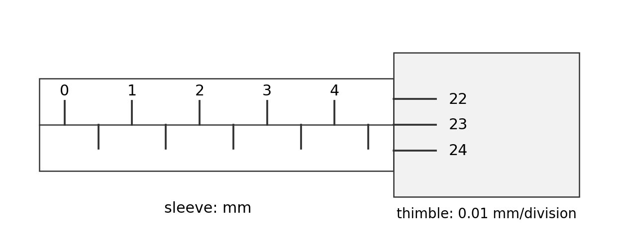
بالنسبة للميكرومتر، أضف قراءة الأكمام الظاهرة وقراءة الطرمبل. شمل علامة النصف مليمتر الظاهرة على الأكمام عند الاقتضاء. استخدم المفتاح الدوار لتطبيق ضغط تماس متناسق، بدلاً من شد الأفواه بشدة مفرطة.
بالنسبة للكيسير، اقرأ المقياس الرئيسي مباشرة قبل الصفر العديدي، ثم أضف التقسيم العديدي المصابح مضروباً في دقته. تحقق من أن أفواه الكيسير تلامس الأسطح المقصودة دون ميلان. لا تستنتج مقياساً مفقوداً من وصف نصي مستخرج: اقرأ رسم الأداة نفسه.
اقرأ الأكمام قبل إضافة تقسيم الطرمبل المصابح.
مثال محلول. آخر علامة مرئية على الكمّاس هي $4.5\ \text{mm}$. انقسام الإصبع 23 يتوافق مع خط المرجع. الدقة هي $0.01\ \text{mm}$ والخطأ الصفري هو $+0.02\ \text{mm}$.
تجنب المنظر عن طريق النظر إلى المقياس على طول خط البصر الصحيح. استخدم مثلثاً للزوايا لنقل ارتفاع أو موقع إلى مسطرة. حافظ على المسطرة موازية للمسافة المقاسة؛ فالمسطرة المائلة تقيس مسافة مختلفة.
البوابة الضوئية تقيس وقت الحجب لجسم يعيق الحركة. بطول حجب معروف $l$، تكون السرعة $v=l/t$. هذا يعطي السرعة أثناء المرور، وليس التسارع بمفرده. لإيجاد التسارع، قس تغير السرعة خلال زمن معروف، أو استخدم معادلة حركة مبررة مع كميات مقاسة إضافية. لا تسمِّ $l/t$ تسارعاً.
يمكن لفيديو بمعدل إطارات معروف أن يقلل من عدم اليقين في زمن التفاعل. عُد الإطارات بين أحداث البداية والنهاية المحددة بوضوح، ثم استخدم $t=N/f_{\text{frame}}$. يحدد فترة الإطار دقة القياس الزمني. لا تزال الصور المموهة أو مواقع الأحداث غير الواضحة قد تُحد من النتيجة.
الجداول والأرقام المعنوية
ضع الكمية والوحدة معاً في عنوان كل عمود، على سبيل المثال $l/\text{mm}$. سجّل القياسات الخام بأماكن عشرية تطابق دقة الأداة. لا تضيف أرقاماً إضافية لا تستطيع الأداة تمييزها.
القراءة
الزمن / ث
1
5.12
2
5.24
3
5.18
4
5.20
كل هذه القيم لها نفس المكانين العشريين. يمكن الاحتفاظ بالمتوسط المحسوب بأرقام إضافية أثناء الحساب، ثم الإبلاغ عنه بشكل مناسب. عادةً ما تُعطى القيم المعالجة للرسم بيانيًا بثلاثة أرقام معنوية، إلا إذا تطلبت السؤال أو البيانات خلاف ذلك. لا تخلط بين $5.1$ و$5.24$ و$5.180$ وكأنها جاءت من عرض واحد لم يتغير.
القراءة الشاذة لا تتناسب مع النمط. تحقق من القراءة وطريقة القياس وأعد القياس إن أمكن. لا تحذف القيمة الأقل ملاءمة بصمت. أي شذوذ مشتبه به يحتاج إلى سبب وقرار مسجل.
عدم اليقين في هذه الوحدة
لقراءة واحدة، تستخدم هذه المواصفات نصف دقة الأداة كتقدير أساسي لعدم اليقين المطلقة. هذا لا يعني أن الدقة هي المصدر الوحيد لعدم اليقين. قد تجعل نقطة النهاية غير المعرفة بوضوح، أو زمن التفاعل، أو المحاذاة عدم اليقين أكبر.
أبلغ عن حوالي $(5.19\pm0.06)\ \text{s}$. احتفظ بالمتوسط غير المدور في حساب النسبة المئوية. انتشار التكرار أكبر بكثير من نصف جزء من百分 ثانية، لذا فإن اقتباس دقة العرض وحده سيخفي التباين الملاحظ.
الوحدة 3 لا تتطلب تركيب عدمات اليقين المئوية في كمية محسوبة. إذا تم تزويدك بعدم يقين لتلك الكمية، فاستخدمه مباشرة. لا تقدم قاعدة نشر متقدمة كمتطلب هنا.
الرسوم البيانية ومعالجة النتائج
اختر مقياسات تعرض البيانات
حدد أي كمية تنتمي إلى كل محور. استخدم تسميات واضحة للكمية/الوحدة ومقاييس منتظمة. استخدم جزءًا كبيرًا من الشبكة المتاحة؛ تجنب الفواصل الصعبة التي يصعب تقسيمها. لا يجب أن يبدأ كل محور دائمًا عند الصفر، ولكن لا تخف ما إذا كانت علاقة تناسب مقترحة تمر عبر نقطة الأصل.
ضع علامات صليب صغيرة بدقة. ارسم خط ميل مفضل أو منحنى أملس بناءً على العلاقة. لا تربط النقاط المتذبذبة بخط متعرج إلا إذا طلب السؤال ذلك. يجب أن يوازن الخط المستقيم المفضل التشتت بدلاً من المرور عبر كل نقطة.
استخدم نقاطاً بعيدة على خط الميل المفضل، وليس زوجاً صغيراً من نقاط البيانات المجاورة.
تحويل الميل إلى ثابت فيزيائي
بالنسبة لخط $y=mx+c$، حدد أي جزء من المعادلة الفيزيائية يطابق $m$ و$c$. لا يثبت الخط المستقيم التناسب المباشر إذا كان التقاطعه غير صفري.
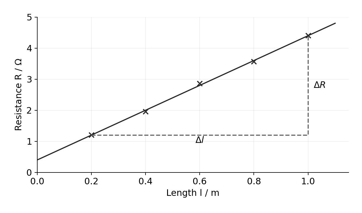
مثال محلول. سلك يتبع $R=(\rho/A)l+R_0$. يمر خط ميل مفضل عبر $(0.20\ \text{m},1.20\ \Omega)$ و$(1.00\ \text{m},4.40\ \Omega)$.
معلوم: نقطتان متباعدتان على الخط الملائم. السبب: الميل يساوي $\rho/A$.
إذا كانت $A=1.0\times10^{-7}\ \text{m}^2$، فإن المقاومة النوعية هي:
$$\rho = mA = 4.00\ \Omega\,\text{m}^{-1}\times1.0\times10^{-7}\ \text{m}^2 = 4.0\times10^{-7}\ \Omega\,\text{m}$$
قد يمثل التقاطع الثابت مقاومة التلامس أو الأسلاك. قسمة قيمة $R$ المقاسة الواحدة على $l$ ستشمل هذا الانحراف وتعطي ميلاً خاطئاً.
عوامل القياس تنتمي إلى الميل
افتترض أن محوراً مُسمى بـ $f/\text{MHz}$. يكون للميل المقروء من هذا الرسم البياني وحدة MHz. حوّلها إلى Hz قبل استخدام الثوابت SI. الرسم البياني لـ $f$ مقابل $\sin\theta$ له محور أفقي بلا أبعاد؛ لذا يكون لميله وحدات تردد. استخدم وضع الدرجات إذا كانت الزاوية المقاسة بالدرجات.
إذا كانت المعادلة المقدمة $f=(v/\lambda)\sin\theta$، فإن الرسم البياني لـ $f$ مقابل $\sin\theta$ يكون له ميل $v/\lambda$. أعد ترتيب $v=\lambda\times\text{gradient}$. لا تفترض أن كل رسم بياني للتردد له ميل يساوي السرعة.
المنحنيات والذروات والتحسينات المحددة
النطاق الواسع أولاً يحدد الذروة. ثم خذ قراءات أكثر تقارباً حول تلك المنطقة. تكرار نقطة واحدة لا يحدد الذروة بين النقاط الموجودة. حافظ على بقية الظروف ثابتة، واعتبر التشتت عند ذكر أفضل زاوية أو مقاومة.
بالنسبة لتجربة حركة، يمكن لمثلث قائم الزاوية تحسين قياس المسافة الأفقية. بالنسبة لتجربة مصباح، يمكن للحجرة المظلمة تقليل إضاءة الخلفية المتغيرة. بالنسبة لتجربة رنين، اقترب من الصوت الأعلى من كلا الاتجاهين (ترددات أعلى وأقل) وأعد القياس. يستهدف كل تحسين قيداً محدداً.
استنتاجات مدعومة بعدم اليقين
القيمة التي تحتوي على عدم اليقين تصف مجالاً. قارن ذلك المجال بالقيمة المقترحة، ثم اذكر ما تدعمه الأدلة. الاتفاق ضمن حدود عدم اليقين لا يثبت أن المادة أو النموذج تم تحديدهما بشكل فريد.
مثال محلول. الكثافة المقاسة هي $8.90\ \text{g cm}^{-3}$ مع عدم يقين نسبي $0.9\%$. هل يمكن أن تتفق مع القيمة المقترحة $8.94\ \text{g cm}^{-3}$؟
المجال هو تقريباً من $8.82$ إلى $8.98\ \text{g cm}^{-3}$. تقع القيمة المقترحة داخله، لذا تكون القياس متوافقاً مع تلك القيمة. لا يثبت ذلك أن الجسم له ذلك التركيب.
إذا كانت تنبؤات نموذجين تقع كلاهما داخل المجال، فإن البيانات لا تفرق بينهما. قلل عدم اليقين السائد أو أضف قياساً مختلفاً قبل الادعاء بتحديد فريد.
تحقق من نفسك
قبل محاولة حل مسألة عملية كتابية، تأكد من قدرتك على:
تحويل أسماء الأجهزة إلى طريقة قابلة للتطبيق مع ضوابط ومسار معالجة;
قراءة الدقة وتصحيح انزياح الصفر المعروف;
التمييز بين الدقة، والانتظام، وقابلية التكرار، وقابلية الاستنساخ;
حساب المتوسط، ونصف المدى، والشك المئوي;
رسم البيانات، واستخدام مثلث ميل كبير وتفسير نقطة التقاطع;
تحويل الشك المرفق إلى فترة وإعطاء استنتاج مبرر;
ربط كل تحسين بالمشكلة القياسية التي تقللها فعلياً.
Pearson Edexcel IAL Physics WPH14/01، الإصدار 3 (يوليو 2021)، مطبوع ص28–ص31 (PDF ص32–ص35).
إعادة صياغة وفاء للحلقات الرئيسية للمتطلبات المرقمة؛ تطبيع الرموز الرياضية من PDF الأصلي. حدود الأوراق المحلية ليست عناوين محددة رسمية.
فهم واستخدام الدفع FΔt = Δp (القانون الثاني لنيوتن).
الممارسة العملية الأساسية 9: استقصاء القوة المؤثرة على جسم وتغير زخمه.
تطبيق حفظ الزخم الخطي في بعدين.
الممارسة الأساسية 10: استخدام تكنولوجيا المعلومات والاتصالات لتحليل التصادمات بين الكرات الصغيرة، مثل كرات المحامل على سطح طاولة.
تحديد ما إذا كان التصادمرنوعاً مرناً أو غير مرن.
اشتقاق واستخدام E_k = p²/(2m) لجسيم غير نسبي.
المصدر: منهج كامبريدج الدولي
4.2الحركة الدائرية (العبارات 87–91)
Pearson Edexcel IAL Physics WPH14/01، الإصدار 3 (يوليو 2021)، مطبوع ص28–ص31 (PDF ص32–ص35).
إعادة صياغة وفاء للحلقات الرئيسية للمتطلبات المرقمة؛ تطبيع الرموز الرياضية من PDF الأصلي. حدود الأوراق المحلية ليست عناوين محددة رسمية.
التعبير عن الإزاحة الزاوية بالراديان والدرجات، والتحويل بينهما.
فهم السرعة الزاوية واستخدام v = ωr و ω = 2π/T.
استخدام المخططات المتجهية لاشتقاق a = v²/r = rω² واستخدام هذه المعادلات.
فهم أن قوة الجذب المركزية المحصلة تُنتج وتُحافظ على الحركة الدائرية.
استخدام F = ma = mv²/r = mrω².
المصدر: منهج كامبريدج الدولي
4.3المجالات الكهربائية والجهد (عبارات 92–99)
Pearson Edexcel IAL Physics WPH14/01، الإصدار 3 (يوليو 2021)، مطبوع ص28–ص31 (PDF ص32–ص35).
إعادة صياغة وفاء للحلقات الرئيسية للمتطلبات المرقمة؛ تطبيع الرموز الرياضية من PDF الأصلي. حدود الأوراق المحلية ليست عناوين محددة رسمية.
تعريف المجال الكهربائي بأنه منطقة يخضع فيها جسيم مشحون لقوة.
تعريف شدة المجال الكهربائي E = F/Q واستخدامها.
استخدام قانون كولوم F = Q₁Q₂/(4πε₀r²).
استخدام E = Q/(4πε₀r²) لشحنة نقطية.
فهم العلاقة بين المجال الكهربائي والجهد.
استخدام E = V/d للألواح المتوازية.
استخدام V = Q/(4πε₀r) للمجال الشعاعي.
رسم وقراءة خطوط المجال والأسطح المكافئة للمجالات المنتظمة والشعاعية.
المصدر: منهج كامبريدج الدولي
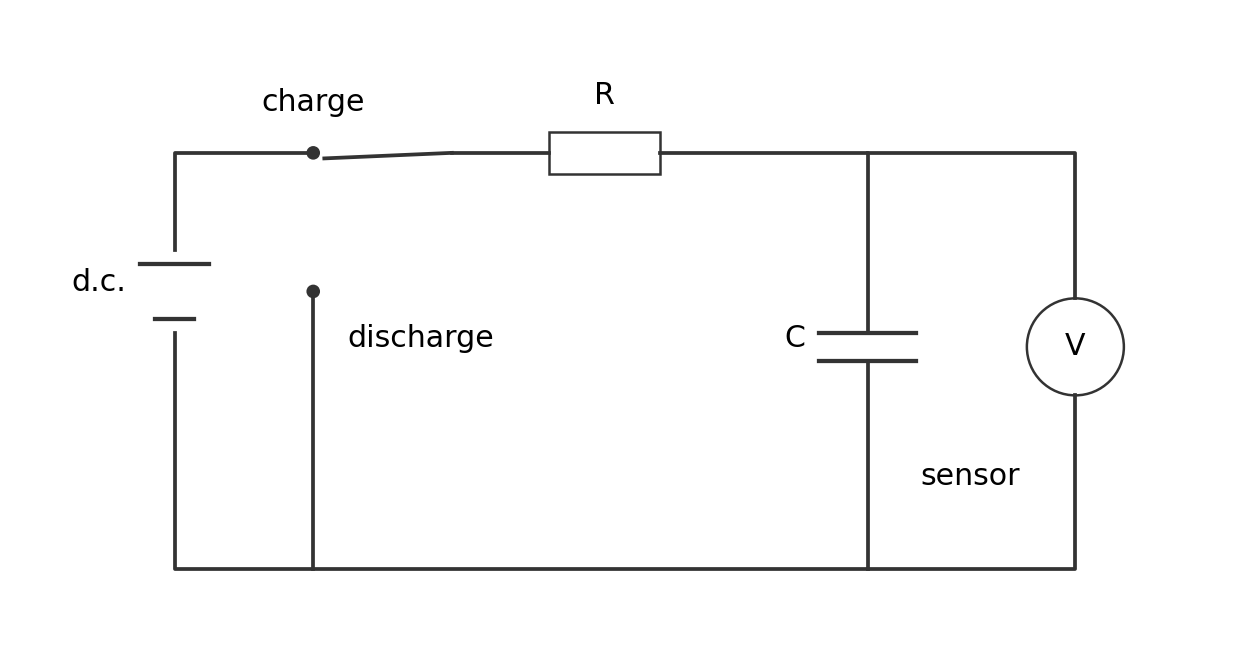
4.4المكثفات ودوائر RC (العبارات 100–104، CP11)
Pearson Edexcel IAL Physics WPH14/01، الإصدار 3 (يوليو 2021)، مطبوع ص28–ص31 (PDF ص32–ص35).
إعادة صياغة وفاء للحلقات الرئيسية للمتطلبات المرقمة؛ تطبيع الرموز الرياضية من PDF الأصلي. حدود الأوراق المحلية ليست عناوين محددة رسمية.
عرّف السعة C = Q/V واستخدم المعادلة.
اشتق الطاقة المخزنة W = ½QV من المساحة تحت منحنى فرق الجهد–الشحنة؛ اشتق واستخدم W = ½CV² و W = Q²/(2C).
ارسم ومنحنى شحن/تفريغ المقاومة–المكثف وأفسره، وافهم ثابت الزمن RC.
التمرين العمائي الأساسي 11: استخدم راسم تذببات أو مسجل بيانات لعرض وتحليل فرق جهد المكثف أثناء الشحن والتفريغ عبر مقاومة.
استخدم Q = Q₀ exp(−t/RC)؛ اشتق واستخدم معادلات التيار وفرق الجهد المقابلة وأشكالها اللوغاريتمية.
المصدر: منهج كامبريدج الدولي
4.5القوى المغناطيسية والحث (العبارات 105–110)
English
Pearson Edexcel IAL Physics WPH14/01, Issue 3 (July 2021), printed pp.28–31 (PDF pp.32–35).
Main-loop faithful paraphrase of numbered requirements; mathematical notation normalised from the original PDF. Local sheet boundaries are not official specification headings.
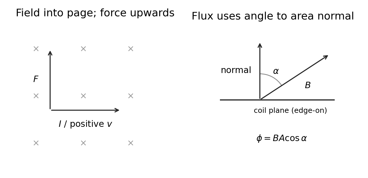
Understand magnetic flux density B, flux φ and flux linkage Nφ.
Use F = Bqv sinθ and apply Fleming's left-hand rule to charged particles.
Use F = BIl sinθ and apply Fleming's left-hand rule to conductors.
Understand what affects induced e.m.f. when a coil and permanent magnet move relatively.
Understand what affects induced e.m.f. when current changes in another linked coil.
Use Faraday's law and the combined Faraday–Lenz equation e.m.f. = −d(Nφ)/dt.
المصدر: منهج كامبريدج الدولي
4.6البنية النووية والمسرعات والمسارات (العبارات 111–117، 120)
English
Pearson Edexcel IAL Physics WPH14/01, Issue 3 (July 2021), printed pp.28–31 (PDF pp.32–35).
Main-loop faithful paraphrase of numbered requirements; mathematical notation normalised from the original PDF. Local sheet boundaries are not official specification headings.
Understand nucleon (mass) number and proton (atomic) number.
Explain large-angle alpha-scattering evidence for the nuclear model and the historical change in atomic models.
Understand thermionic electron emission and acceleration using electric and magnetic fields.
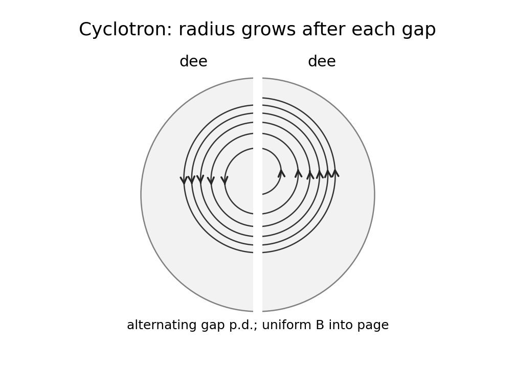
Understand electric/magnetic fields in linacs, cyclotrons and detectors; detector detail limited to ionisation and deflection principles.
Derive and use r = p/(BQ) for a charged particle in a magnetic field.
Apply charge, energy and momentum conservation to particle interactions and interpret tracks.
Explain why high energies are needed to investigate nucleon structure.
Understand significant relativistic increases in particle lifetime; relativistic equations are not required.
Pearson Edexcel IAL Physics WPH14/01، الإصدار 3 (يوليو 2021)، مطبوع ص28–ص31 (PDF ص32–ص35).
إعادة صياغة وفاء للحلقات الرئيسية للمتطلبات المرقمة؛ تطبيع الرموز الرياضية من PDF الأصلي. حدود الأوراق المحلية ليست عناوين محددة رسمية.
استخدام ΔE = c²Δm في إنشاء وجسيمات مضادة ومادة/مادة مضادة.
استخدام MeV/GeV للطاقة وMeV/c² أو GeV/c² للكتلة والتحويل إلى النظام الدولي (SI).
تصنيف الباريونات (ثلاث كواركات)، والميزونات (كوارك/أنتيكوارك)، والليبتونات الأساسية والفوتونات؛ معرفة أن تناظر النموذج قد تنبأ بكوارك القمم.
استخدام خصائص الجسيم لاستنتاج الخصائص المقابلة للجسيم المضاد والعكس.
استخدام حفظ الشحنة، ورقم الباريون، ورقم الليبتون لتقييم التفاعلات.
كتابة وتفسير معادلات الجسيم من الرموز المقدمة.
المصدر: منهج كامبريدج الدولي
ورقة عمل
English
From a collision to a particle accelerator
A car bumper and a particle detector seem very different. Both use momentum and forces. This unit follows those ideas into circular motion, electric fields, magnetic fields and particle interactions.
WPH14 assesses requirements 81–124 of the Issue 3 specification. It can also use knowledge from Units 1–2. Use the seven skill sheets in order. Check units, directions and the assumptions behind each equation. A familiar equation can give a wrong answer when its model does not fit.
Impulse and two-dimensional collisions
Force changes momentum
Momentum 动量 is the vector $\mathbf p=m\mathbf v$. Choose a positive direction before using signs. Impulse 冲量 is the change in momentum. For constant force, or the average force over an interval:
$$F_{\text{average}}\Delta t=\Delta p=m(v-u)$$
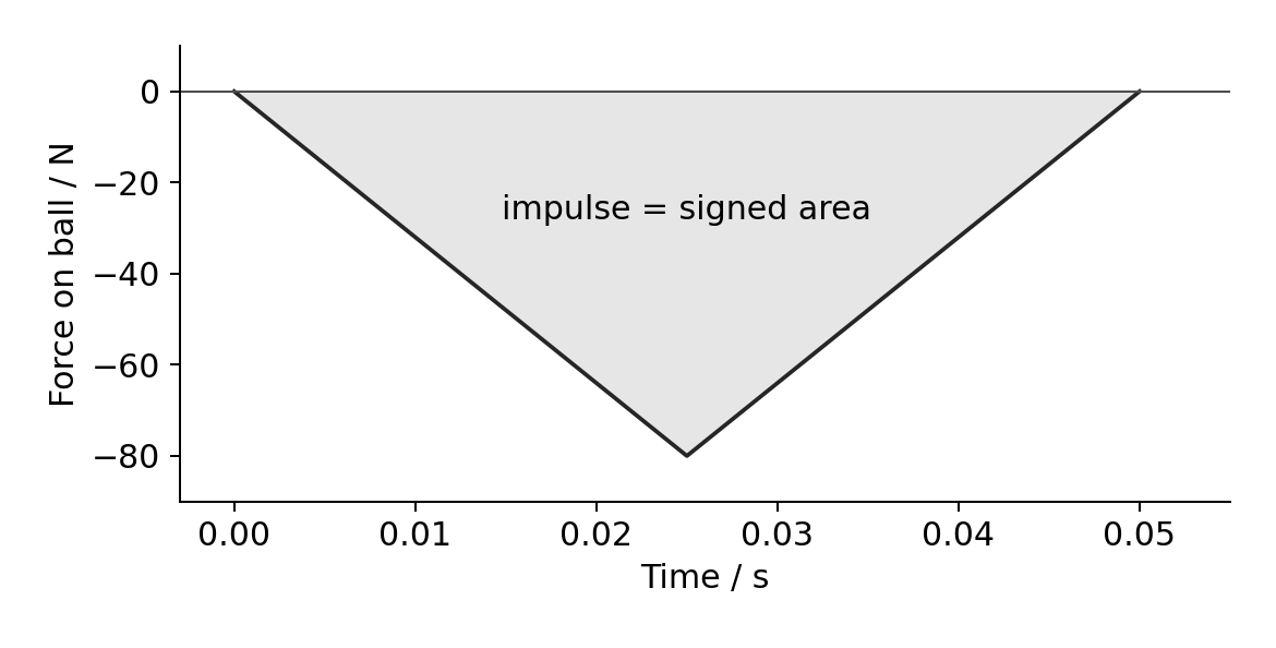
A changing force gives an impulse equal to the signed area under its force–time graph. A triangular pulse has area $\frac12\times\text{base}\times\text{height}$. An area below the time axis is negative. The maximum force is not automatically the average force.
Worked example. A $0.20\ \text{kg}$ ball approaches a wall at $+6.0\ \text{m s}^{-1}$. It rebounds at $-4.0\ \text{m s}^{-1}$. Contact lasts $0.050\ \text{s}$. Find average force on the ball.
Known: mass, signed initial/final velocities and contact time.
Why: force impulse changes the ball's momentum; rebound reverses the sign.
$$\Delta p=m(v-u)=0.20\ \text{kg}\times(-4.0-6.0)\ \text{m s}^{-1}=-2.0\ \text{kg m s}^{-1}$$
$$F_{\text{average}}=\frac{\Delta p}{\Delta t}=\frac{-2.0\ \text{kg m s}^{-1}}{0.050\ \text{s}}=-40\ \text{N}$$
The force is opposite the chosen positive direction. The wall feels an opposite force. A deforming bumper or helmet increases stopping time. For the same momentum change, this reduces average force. It does not remove the momentum change.
Conserve each momentum component
An isolated system 孤立系统 has no significant external impulse during the event. Its total momentum is conserved. Internal forces cancel in opposite pairs. Momentum conservation does not require kinetic energy conservation.
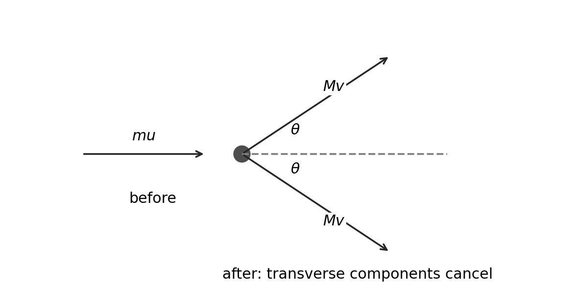
For a collision in a plane, resolve every momentum into two perpendicular axes:
Use the angle measured from the chosen axis. Include signs; a downward component is negative if upwards is positive. Do not add momentum magnitudes when directions differ.
Worked example. A $0.10\ \text{kg}$ sphere moving at $2.0\ \text{m s}^{-1}$ strikes two stationary spheres, each $0.10\ \text{kg}$. It stops. The two others leave symmetrically at $1.2\ \text{m s}^{-1}$, at angles $+\theta$ and $-\theta$ to the original direction. Find their separation angle and classify the collision.
Why: transverse momenta cancel by symmetry; longitudinal momentum gives $\theta$.
An elastic collision 弹性碰撞 conserves total kinetic energy as well as momentum. An inelastic collision 非弹性碰撞 does not conserve kinetic energy; some becomes other forms of energy.
This collision is inelastic. Total energy is still conserved. In an ordinary passive collision, kinetic energy cannot increase without an additional energy source.
For a non-relativistic particle 非相对论粒子, use $p=mv$ and $E_k=\frac12mv^2$. Substituting $v=p/m$ gives:
At equal kinetic energy, $p=\sqrt{2mE_k}$: a larger mass has larger momentum. At equal momentum, a larger mass has smaller kinetic energy. These equations are not valid for a particle moving close to light speed.
Core practicals 9 and 10
For core practical 9, use a trolley, force sensor and data logger. Measure trolley mass and velocities just before/after contact using light gates or a motion sensor. Record the force–time pulse at a sampling rate fast enough to resolve it. Zero the force sensor; use consistent axes for force and velocity. Integrate the graph area and compare it with $m(v-u)$. Repeat for different contact forces or speeds. A graph of impulse against momentum change should have gradient close to one. Friction, sensor offsets and missed parts of the pulse can cause disagreement. Secure the track and catch the trolley safely.
For core practical 10, record small spheres colliding on a level surface using an overhead camera. Include a length scale in the collision plane and a known frame rate. Keep the camera perpendicular to reduce perspective error. Track centres over several frames before and after the short collision. Convert pixel displacements to metres and frame intervals to seconds. Determine both velocity components, then compare total momentum components and kinetic energies. Repeat with different approach directions. Include uncertainty from positions, timing and scale calibration. A small mismatch within uncertainty is not evidence that momentum fails. Keep spheres contained so they cannot fall or become a slipping hazard.
Circular motion
Angle, angular speed and tangential speed
An angle of one radian 弧度 subtends an arc equal to the radius. Hence $\theta=s/r$, with angle in radians. One revolution is $2\pi$ radians or $360^\circ$.
Angular velocity 角速度 describes the rate of angular displacement. In the plane problems here, use its signed rotational rate or magnitude as appropriate. Points on one rigid turntable have the same angular speed. Points farther from its centre have larger tangential speed 切向速率. Their velocity directions also vary around the circle.
Worked example. A wheel rotates at $120$ revolutions per minute. Find angular speed and acceleration of a point $0.25\ \text{m}$ from its centre.
Keep the unrounded angular speed during the calculation. Use radius, not diameter.
Why acceleration points inward
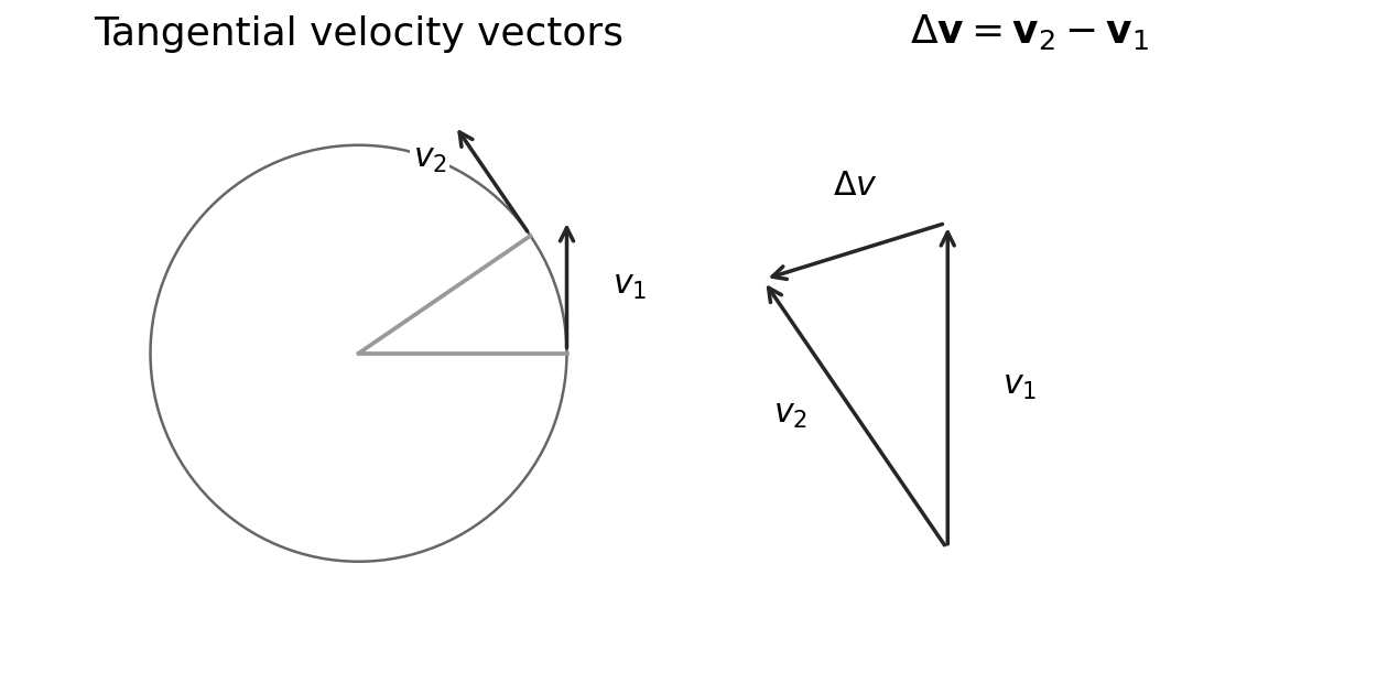
Uniform circular motion has constant speed but changing velocity. Draw the initial and final tangential velocity vectors. The change is $\Delta\mathbf v=\mathbf v_2-\mathbf v_1$, not their sum. For a small angular change, the velocity triangle and radius triangle are similar:
Centripetal force names the resultant of real forces. It is not an extra force to add to a force diagram. Friction can provide it on a turntable. Tension can provide it for a ball on a string.
Write the real-force equation
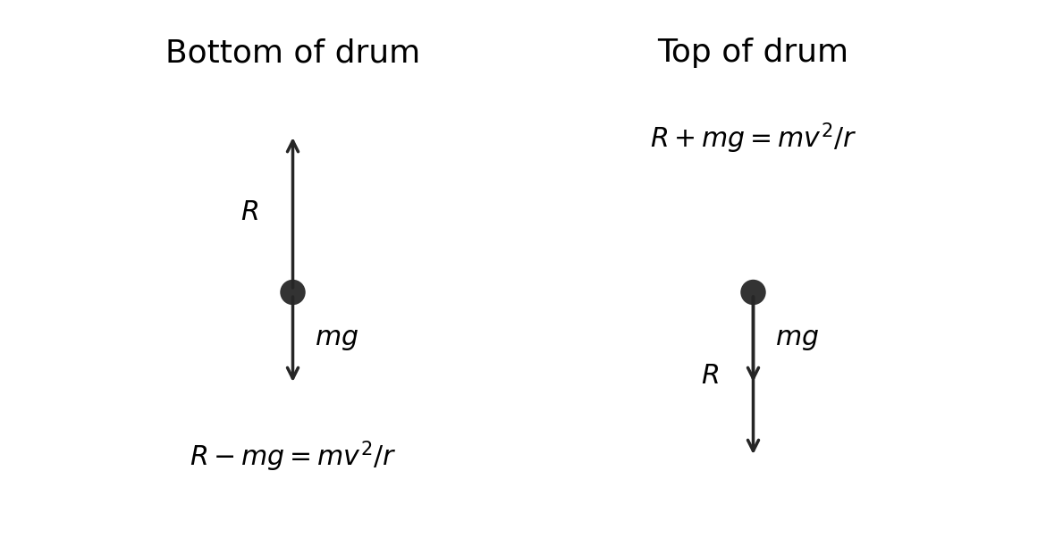
For clothing against the inside of a vertical drum, weight always points down. The drum's normal reaction points towards the centre. At constant speed:
The required resultant has the same magnitude, but the reaction is larger at the bottom. If contact is lost, the surface cannot provide a pulling normal reaction. Check this before using a circular-path model.
For a horizontal turntable, the largest available friction must be at least $mr\omega^2$. If maximum friction is $mg/25$:
Mass cancels because both required and available forces scale with mass. If the inward force disappears, motion initially follows the tangent. Gravity can then curve the later path; “tangent” describes the release direction.
Electric fields and potential
Force and potential describe different things
An electric field 电场 is a region where a charged particle experiences a force. Electric field strength 电场强度 is force per unit positive test charge:
Potential is a scalar; field is a vector. A point with zero potential need not have zero field. Adding signed potentials is different from adding field vectors.
Radial and uniform fields
For point charges, or outside an isolated charged conducting sphere, with $k=1/(4\pi\varepsilon_0)$:
Here $r$ is separation of charge centres; sphere distances are measured from its centre. Like charges repel, unlike charges attract. Potential takes the sign of $Q$ when zero is at infinity.
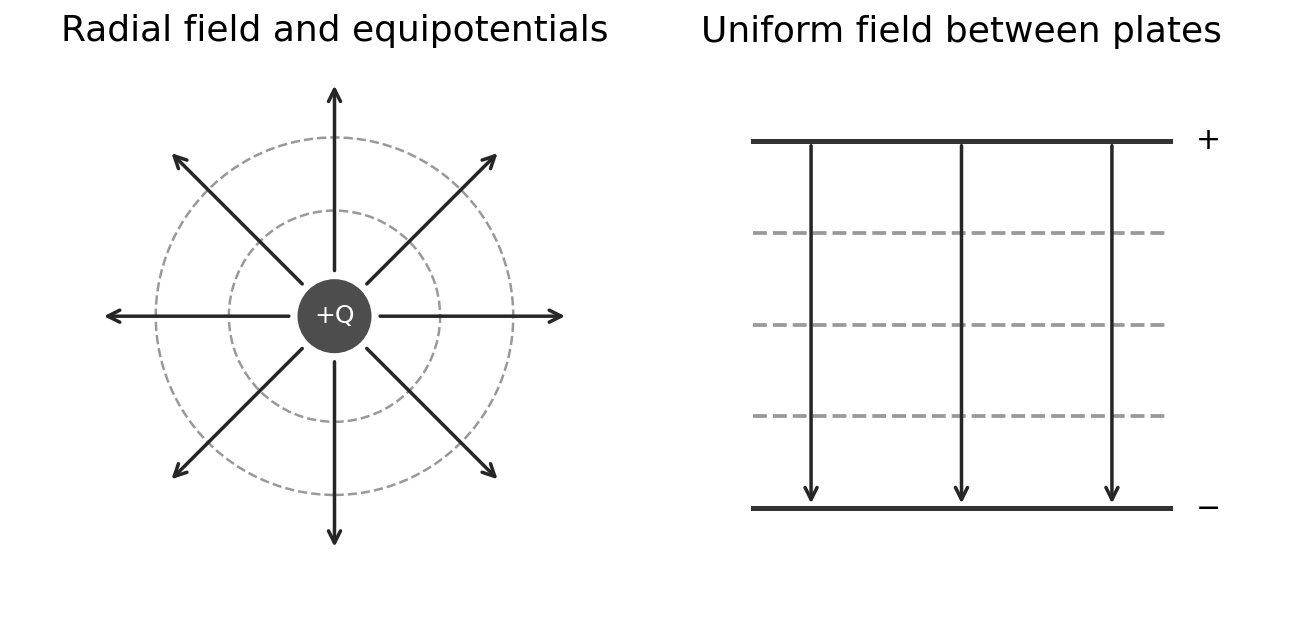
Between large parallel plates, away from edges, the field is approximately uniform:
$$|E|=\frac{|\Delta V|}{d}$$
The field points from higher to lower potential. Plate separation $d$ is perpendicular to the plates. An equipotential 等势面 has the same potential everywhere. Field lines cross equipotentials at right angles. Moving along one involves no change in electric potential energy.
The radial field is the negative potential gradient: $E_r=-\mathrm dV/\mathrm dr$. For a positive source, the signed area under its $E$–$r$ curve from $r$ to infinity equals $V(r)$. The area from zero to $r$ is not that potential. In a uniform field, closer equally spaced potential levels mean stronger field.
Worked example. A sphere of radius $0.20\ \text{m}$ has potential $9.0\ \text{kV}$. Find charge and field at $0.30\ \text{m}$ from its centre. Use $k=8.99\times10^9\ \text{N m}^2\text{C}^{-2}$.
Use the surface radius to find charge, then the new centre-distance to find field. Do not reuse the surface distance for the second step.
Compare electrical and gravitational forces
A stationary charged oil drop can satisfy $|q|E=mg$. Use $m=\rho\mathcal V$ if density and volume are given. Divide the charge magnitude by $e=1.60\times10^{-19}\ \text{C}$ to test whether it is close to an integer multiple. Charge sign follows the direction of force required, not its magnitude alone.
To lift a spherical grain, compare $qE$ with $\rho(4\pi r^3/3)g$. Radius is half the listed diameter. A calculated maximum diameter is a threshold: choose the largest listed diameter below it. On an inclined panel, the normal component of weight is $mg\cos\theta$. The electric force perpendicular to the panel need overcome that component to detach a grain; gravity also has a downslope component.
Capacitors and RC circuits
Charge storage and energy
A capacitor 电容器 stores separated charge on two conductors. They carry equal and opposite charges in the ideal two-plate model. The quoted charge $Q$ is the magnitude on either plate, not the sum of both magnitudes. Capacitance 电容 is charge stored per unit p.d.:
$$C=\frac QV$$
One farad is one coulomb per volt. For constant capacitance, a $V$–$Q$ graph is straight through the origin with gradient $1/C$. Its area gives the work needed to transfer charge onto the capacitor:
$$W=\frac12QV=\frac12CV^2=\frac{Q^2}{2C}$$
The factor one half appears because p.d. rises from zero while charge is transferred. It is not $QV$ at the final voltage throughout charging. For discharge between non-zero voltages, subtract the two stored energies:
This is different from $\frac12C(V_{\text{initial}}-V_{\text{final}})^2$.
Charging and discharging
In an ideal series resistor–capacitor charging circuit, initially uncharged, the capacitor p.d. is zero. The resistor initially has the full supply p.d., so current is maximum. As charge builds, capacitor p.d. rises. Resistor p.d. and current fall. At full charge, current is zero and capacitor p.d. equals supply p.d.
For discharge through a fixed resistance, use signed current consistently or work with its magnitude:
The voltage relation follows from $Q=CV$ with constant $C$. Current magnitude follows from $|I|=V/R$ with constant $R$. The time constant 时间常数 is $\tau=RC$. After one time constant, $Q$, $V$ and current magnitude are $e^{-1}\approx0.368$ of their initial values. After three time constants they are about $5\%$, not zero. Stored energy falls faster because it depends on $V^2$.
A charging capacitor voltage rises towards $V_s$; charging current falls towards zero. Do not sketch the same curve for both quantities. Equal $V_C$ and $V_R$ means each is $V_s/2$, reached at $t=RC\ln2$.
Taking natural logs of the discharge equation gives:
$$\ln V=\ln V_0-\frac{t}{RC}$$
Thus a graph of $\ln V$ against $t$ has gradient $-1/(RC)$ and intercept $\ln V_0$. The same forms hold for $Q$ and current magnitude. Use consistent measurement units inside the logged numerical values.
Worked example. A $100\ \mu\text{F}$ capacitor discharges from $12.0\ \text{V}$ through $20.0\ \text{k}\Omega$. Find p.d. after $3.0\ \text{s}$ and energy lost.
The lost stored energy becomes mainly heat in the discharge resistance. Use unrounded voltage in the final calculation.
Core practical 11 and useful extensions
Use a low-voltage d.c. supply, resistor, capacitor and switch. Charge through the resistor, then disconnect the supply and discharge through the known resistance. Connect a voltage sensor, data logger or oscilloscope across the capacitor. Record time and p.d.; choose a sampling interval short compared with $RC$. Use an instrument input resistance large compared with the discharge resistance, otherwise it changes the discharge path.
Keep $R$ and $C$ fixed, repeat after restoring the same initial charge, and compare measured curves with exponential predictions. Determine $RC$ from the $1/e$ level or a log-fit gradient. Avoid taking logs of readings near zero where relative uncertainty is large. For a resistance-tolerance test, calculate $R=-\Delta t/[C\ln(V_2/V_1)]$ during one uninterrupted discharge and compare with both limits of the permitted interval.
Use correct polarity for an electrolytic capacitor and remain below its voltage rating. Discharge it safely through a resistor before altering connections; do not short a charged capacitor. Leakage, sensor loading and resistor heating can change the measured curve.
A smoothing capacitor charges near supply peaks and discharges into the load between them. A smaller load resistance gives a smaller time constant, faster discharge and less smoothing. For two identical series capacitors, the same magnitude of charge appears on each. Their equal p.d.s share the supply, so each stores half the charge of one identical capacitor connected alone. This sharing is a useful bridge to the selected paper; it does not replace the main capacitance model.
Magnetic forces and induction
Directions, flux and force
Magnetic flux density 磁感应强度$B$ describes the field's force effect. For a straight wire of length $l$ in a uniform field:
$$F=BIl\sin\theta$$
Here $\theta$ is between conventional current and field. Only the length inside the field counts. For one charged particle:
$$F=|q|vB\sin\theta$$
Use Fleming's left-hand rule 弗莱明左手定则: first finger along field, second along conventional current, thumb gives force. A positive charge moves with conventional current. Reverse the result for an electron's motion. Dot symbols mean out of the page; crosses mean into it.
Magnetic force is perpendicular to velocity, so it changes direction without doing work. It cannot, alone, increase the particle's kinetic energy. If $\mathbf v$ is parallel to $\mathbf B$, magnetic force is zero.
Magnetic flux 磁通量 through a flat area in a uniform field is:
$$\phi=BA\cos\alpha$$
Here $\alpha$ is between field and the area's normal, not the plane itself. The unit is the weber. Flux linkage 磁通链 is $N\phi$ when the same flux links each of $N$ turns.
Worked example. A coil has 40 turns and radius $0.015\ \text{m}$. A uniform $0.020\ \text{T}$ field is perpendicular to its plane. Find flux linkage.
Use radius, not diameter, and multiply by turns only when finding linkage. A balance under magnets measures the opposite reaction to a force on a separately supported wire. Convert a balance reading change $\Delta m$ to force $\Delta mg$, not $\Delta m$ itself.
A changing linkage induces an e.m.f.
Electromagnetic induction 电磁感应 occurs when flux linkage changes. Relative movement of a coil and magnet can cause it. Rotating the coil or changing current in another linked coil can also cause it. A stationary coil in a constant field has no induced e.m.f. merely because flux is present.
Faraday's law 法拉第电磁感应定律 relates e.m.f. magnitude to rate of flux-linkage change. Lenz's law 楞次定律 gives the opposing direction:
Induced current, if the circuit is closed, produces a magnetic effect opposing the change that caused it. It does not always oppose the existing field: when that field decreases, the induced effect helps maintain it. This opposition is consistent with energy conservation.
Worked example. Flux through each of 50 turns decreases from $6.0\times10^{-5}$ to $2.0\times10^{-5}\ \text{Wb}$ in $0.020\ \text{s}$. Find average induced e.m.f. magnitude.
Faster movement, stronger field, more turns or larger linked area can increase the rate. Explain which quantity actually changes. In a magnetic-strip reader, reversing pole orientation reverses signal direction. For a straight boundary swept across an area of width $L$ at speed $v$, $\Delta A/\Delta t=Lv$, giving $|\mathcal E|=NBLv$ under that uniform-field model.
Wireless charging uses alternating current in one coil, producing changing magnetic field and changing linkage in the phone coil. That induces an e.m.f. The receiving circuit can then charge the battery. Equal turn counts do not ensure equal voltages: some flux may fail to link the other coil, especially with separation or without an iron core.
Nuclear structure, accelerators and tracks
The nucleus and scattering evidence
In $^{A}_{Z}X$, proton number 质子数$Z$ counts protons and nucleon number 核子数$A$ counts protons plus neutrons. The neutron count is $A-Z$. A neutral atom has $Z$ electrons; an ion need not.
The older distributed-positive-charge model could explain small deflections but not the observed rare large-angle alpha scattering. Most alpha particles pass nearly straight through thin foil, showing that most of the atom is empty space. A small fraction experience very large deflections. Positive alpha particles feel strong electrostatic repulsion near a small, dense, positive nucleus containing most atomic mass. Few large-angle events show that the nucleus occupies a small fraction of the atom's volume. Keep each observation linked to the particular conclusion it supports.
Make, accelerate and steer a beam
Thermionic emission 热电子发射 releases electrons from a heated metal. Heating supplies energy so some electrons can leave the surface. A positive accelerating electrode attracts them through a vacuum. A potential difference changes kinetic energy by the electric work:
For speed calculations use the positive energy gain $|q|\,|\Delta V|$ only when the particle is accelerated through the field in the appropriate direction. Starting from rest, well below light speed:
$$\frac12mv^2=|q|\,|\Delta V|$$
A linear accelerator 直线加速器 uses alternating p.d. across gaps between drift tubes. Particles accelerate in gaps and are shielded inside the conducting tubes. The polarity reverses while particles are inside, so the next gap accelerates them again. At constant alternating frequency, increasing speed requires longer tubes to maintain the time between successive gaps. Across $n$ equal accelerating gaps, total kinetic-energy gain is $n|q|V_{\text{gap}}$.
A cyclotron 回旋加速器 uses a magnetic field perpendicular to two hollow dees. Electric field accelerates particles across the gap. Inside a dee, magnetic force curves the path without increasing speed. Polarity reverses during each half-turn, allowing another energy gain at the next crossing. With perpendicular entry:
In the non-relativistic model, the period is independent of speed. Increasing speed increases radius. Time in one dee is $T/2$, not $T$. The formula assumes constant field and fixed mass in this model; synchronisation fails as relativistic effects become important.
Worked example. A proton moves perpendicular to $B=0.40\ \text{T}$ with momentum $2.0\times10^{-20}\ \text{kg m s}^{-1}$. Use proton mass $1.67\times10^{-27}\ \text{kg}$.
When starting instead from a de Broglie wavelength, use $p=h/\lambda$, then $E_k=p^2/(2m)$ and $V=E_k/|q|$. Check that the non-relativistic assumption remains suitable.
Read detector evidence carefully
Charged particles ionise matter along their paths, leaving detectable tracks. A neutral particle does not make a direct ionisation track in this model. Its presence can be inferred from missing momentum or from charged products it later produces.
In a known perpendicular magnetic field, curvature direction together with travel direction can identify charge sign. Without field direction, curvature alone cannot give sign. Radius gives momentum through $p=B|q|r$; comparing radii requires knowledge of charge magnitude. A tightening track often shows momentum being lost. Do not infer travel direction from a constant-radius arc alone.
Conserve charge, total energy and vector momentum at an interaction. If visible outgoing momenta do not add to the incoming momentum, a neutral product may carry the missing component. Draw a vector balance rather than guessing from the number of tracks.
High energies probe nucleon structure in two ways. Large momentum gives a short de Broglie wavelength, allowing small structure to be resolved. High collision energy also allows new massive particles to be created. Quarks are not observed as isolated free particles; do not describe a high-energy collision simply as removing a free quark.
Fast muons can reach the ground because their average lifetime measured in the Earth's frame is increased at speeds close to $c$. This does not mean they exceed light speed. Unit 4 requires the significance of this lifetime increase, not use of relativistic equations.
Particles, antiparticles and conservation
Families and antiparticles
In the quark–lepton model 夸克—轻子模型, baryons and mesons contain quarks. Leptons are fundamental particles in the model.
A baryon 重子 contains three quarks, for example a proton $uud$ or neutron $udd$. An antibaryon contains three antiquarks.
A meson 介子 contains one quark and one antiquark, for example a pion.
A lepton 轻子 is fundamental, for example an electron or neutrino. A positron is an antilepton, not a meson.
A photon is the quantum of electromagnetic radiation; it is neither a baryon nor a lepton.
Up-type quarks have charge $+2e/3$ and down-type quarks $-e/3$. Antiquarks have opposite charges. For example, $uud$ sums to $+e$ and $udd$ to zero. The symmetry of the quark families predicted a top quark before it was observed. Classification models make testable predictions, not just lists of known particles.
An antiparticle 反粒子 has the same rest mass as its particle and opposite electric charge when charged. Other relevant additive quantum numbers also reverse. An electron has lepton number $+1$; its positron has $-1$. Both have baryon number zero. A neutral antiparticle can differ in quantum numbers despite having no electric charge.
Check conserved totals
Assign baryon number $+1$ to a baryon, $-1$ to an antibaryon, and zero to mesons/leptons/photons. Quarks carry $+1/3$ and antiquarks $-1/3$. Assign lepton number $+1$ to a lepton and $-1$ to an antilepton. Compare total charge, baryon number and lepton number on both sides of a proposed reaction. Also check energy and momentum. Passing the listed conservation checks alone does not prove that an interaction will occur; it establishes that those laws do not forbid it.
Worked example. Test $n\rightarrow p+e^-+\bar\nu_e$.
Quantity
Before
After
Charge / $e$
0
$+1-1+0=0$
Baryon number
1
$1+0+0=1$
Lepton number
0
$0+1-1=0$
The antineutrino balances the electron's lepton number. Changing it to a neutrino would make the final total $+2$, so that proposed equation would fail this check. Preserve bars and charge signs when interpreting supplied particle symbols.
Rest energy, creation and annihilation
Mass–energy equivalence 质能等价 relates a rest-mass change to energy:
$$\Delta E=c^2\Delta m$$
In pair production 粒子对产生, energy creates a particle–antiparticle pair. The energy must at least supply both rest masses; extra energy can become kinetic energy or recoil. Momentum must also be conserved, so the surrounding interaction matters. In annihilation 湮灭, particle and antiparticle can turn into photons. A pair initially at rest producing two photons gives equal photon energies and opposite momenta. Each photon carries one particle's rest energy for an equal-mass pair; the total is twice that value.
One electronvolt is $e$ joules: $1\ \text{eV}=1.60\times10^{-19}\ \text{J}$. MeV means $10^6$ eV and GeV means $10^9$ eV. A quoted mass in $\text{MeV}/c^2$ is a mass unit, not an energy unit. Multiply by $c^2$ to get its corresponding rest energy.
Worked example. Convert a mass of $140\ \text{MeV}/c^2$ to kilograms.
Use the same units before comparing masses. Percentage difference from an accepted value is $100\times|m_{\text{predicted}}-m_{\text{accepted}}|/m_{\text{accepted}}$. State the reference value. In threshold questions, distinguish rest-energy supply from kinetic energy; do not use $p=mv$ for a photon or a particle close to $c$.
Check yourself
Can you use signed impulse and two momentum components, then test kinetic energy separately?
Can you derive centripetal acceleration and draw only actual forces?
Can you distinguish field vectors, signed potential and energy changes?
Can you choose the correct capacitor curve and use log slope or tolerance evidence?
Can you explain induction as a change in linkage, including the opposing direction?
Can you separate electric acceleration from magnetic steering and halve a cyclotron period correctly?
Can you preserve particle symbols, conservation totals and energy/mass units?
The skill sheets develop these methods before authentic past-paper tasks. Original practice also covers requirements not sampled in the two recent papers. A short sample of authentic questions does not define the whole syllabus.
الحرارة النوعية/الحرارة الكامنة؛ الطاقة الداخلية؛ التمييز بين انتقال الطاقة ودرجة الحرارة. CP12 مقياس حراري مكافئ/مجزئ جهد وCP13 حرارة كامنة بإدخال كهربائي، فقدان الكتلة وتصحيح الفقدان.
الأدلة المطلوبة عكسياً: plans/2026-10-09-edexcel-ial-physics-u5-demand-map.md. تقييم الوحدة 5 هو تآزري مع الوحدات 1، 2 و4.
الصفر المطلق والكلفن؛ pV=NkT، نسب كمية ثابتة؛ CP14 الضغط/الحجم عند درجة حرارة ثابتة؛ اشتقاق متوسط طاقة الحركة الانتقالية للجزيء 3kT/2 من نظرية الحركة، والتمييز بين سرعة RMS ومتوسط مربع السرعة.
الأدلة المطلوبة عكسياً: plans/2026-10-09-edexcel-ial-physics-u5-demand-map.md. تقييم الوحدة 5 هو تآزري مع الوحدات 1، 2 و4.
فقدان الكتلة والطاقة الرابطة النووية، u والتحويلات SI، الرسم البياني لكل نوكليون والاستقرار، طاقة الاندماج/الانشطار، متطلبات درجة الحرارة والكثافة العالية للاندماج المستدام.
الأدلة المطلوبة عكسياً: plans/2026-10-09-edexcel-ial-physics-u5-demand-map.md. تقييم الوحدة 5 هو تآزري مع الوحدات 1، 2 و4.
محصلة الاستعادة متناسبة وعكسية مع الإزاحة؛ علاقات x,v,a الموقعة والمرحلة، فترات النابض/البندول، ميل المنحنيات، تبادل الطاقة غير المخمدة وفقدان الطاقة المخمدة. CP16 كتلة مجهولة من الترددات الرنانة مع كتل معلومة معايرة.
الأدلة المطلوبة عكسياً: plans/2026-10-09-edexcel-ial-physics-u5-demand-map.md. تقييم الوحدة 5 هو تآزري مع الوحدات 1، 2 و4.
الأدلة المطلوبة عكسياً: plans/2026-10-09-edexcel-ial-physics-u5-demand-map.md. تقييم الوحدة 5 هو تآزري مع الوحدات 1، 2 و4.
المصدر: منهج كامبريدج الدولي
ورقة عمل
English
From an ice pack to a star
An ice pack, a swinging bridge and a distant star all involve energy. This unit links molecular motion, nuclear changes, oscillations and astronomical observations. The task is often to test a claim, not just calculate a number: state the model, carry units through the calculation, then compare your result with the claim.
WPH15 covers statements 125–171 of Pearson Issue 3. It also uses Units 1, 2 and 4. Work through sheets 5.1–5.9 before their matching authentic sets. Use the supplied constants consistently: $g=9.81\ \mathrm{m\,s^{-2}}$, $k_B=1.38\times10^{-23}\ \mathrm{J\,K^{-1}}$ and $G=6.67\times10^{-11}\ \mathrm{N\,m^2\,kg^{-2}}$ unless the question gives a different local value. Here $k_B$ is the Boltzmann constant; $k_s$ denotes a spring constant.
Heating, phase change and thermistor calibration
Follow the energy, not only the temperature
Internal energy 内能 is the total energy in the random motion and interactions of molecules: random kinetic energy plus intermolecular potential energy. It excludes the kinetic energy of the whole object moving together. Temperature relates to average random molecular kinetic energy, not total internal energy. Two samples at the same temperature can have different internal energies because their amounts and states differ.
Specific heat capacity 比热容$c$ is the energy needed per kilogram for a one-kelvin temperature rise without a change of state. Specific latent heat 比潜热$L$ is the energy transferred per kilogram during a particular change of state at constant temperature.
A temperature difference of $1\ ^\circ\mathrm C$ equals a difference of $1\ \mathrm K$. Absolute temperatures in gas and radiation laws must be kelvin. During melting or boiling, energy changes molecular arrangements and potential energy while temperature remains constant in the ideal constant-pressure phase change. An ice pack absorbs energy from the food/surroundings as it melts. It does not send “cold energy” into the food.
At constant heating power, steeper temperature–time gradients mean smaller $mc$, provided heat loss is negligible. A flat section does not mean that energy transfer has stopped. For a heater, input energy is $E_{\rm in}=Pt=VIt$; useful thermal energy can be smaller because energy escapes to surroundings.
Worked example. A $0.40\ \mathrm{kg}$ block of ice at $-10\ ^\circ\mathrm C$ melts to water at $0\ ^\circ\mathrm C$. Use $c_{\rm ice}=2100\ \mathrm{J\,kg^{-1}\,K^{-1}}$ and $L_f=3.4\times10^5\ \mathrm{J\,kg^{-1}}$.
Known: mass, initial/final temperatures and material constants. Why: warming the solid and melting it are separate energy transfers.
Worked example. A $1000\ \mathrm W$ heater boils away $0.20\ \mathrm{kg}$ of water in $600\ \mathrm s$. Find efficiency, using $L_v=2.26\times10^6\ \mathrm{J\,kg^{-1}}$.
For repeated kettle loads, calculate total water volume, number of loads and total operating time. Compare energies over the same stated interval. Standby loss over a day and input needed to boil water are different quantities; state what a particular comparison actually establishes.
CP12: calibrate a thermostat
A thermistor 热敏电阻 has resistance that changes with temperature. The usual negative-temperature-coefficient (NTC) thermistor decreases in resistance when heated. In a potential divider 分压器:
With the thermistor as the lower resistor and output measured across it, warming reduces output voltage. Swapping resistor positions reverses that trend. A thermostat switches at a chosen output threshold; the divider alone is not a complete switching device.
For core practical 12, place the thermistor and a reference thermometer close together in a stirred water bath. Keep electrical contacts dry and insulated. At several temperatures across the intended range, wait for thermal equilibrium and record temperature and divider voltage. Keep supply voltage and fixed resistance unchanged. Use a high-input-resistance voltmeter to reduce loading. Plot output against temperature and interpolate the voltage for the chosen switching temperature. Repeat readings or compare warming/cooling to reveal lag. Do not assume a linear calibration without evidence. Use low-voltage electricity and take care with hot water.
CP13: measure latent heat
Supply measured electrical power to a material during its phase change. Measure mass melted or evaporated over a timed interval after conditions stabilise. A balance measures mass change; do not confuse collected liquid volume with mass. Without loss correction, $L=VIt/\Delta m$ assumes all supplied energy causes the phase change.
A useful correction is to compare two powers at the same steady phase-change temperature. If heat-loss power is approximately unchanged, subtracting the two measurements removes it:
$$L=\frac{P_2-P_1}{\dot m_2-\dot m_1}$$
State that constant-loss assumption. A control measurement of melting without the heater is another possible correction in a suitable ice experiment. Reduce heat loss with insulation where safe; avoid splashing, hot surfaces and unsafe mains connections.
Ideal gases and molecular kinetic energy
Kelvin and the ideal-gas model
Absolute zero 绝对零度 is $0\ \mathrm K$, about $-273\ ^\circ\mathrm C$. It is the lower limit of thermodynamic temperature. In the classical ideal-gas model, average translational kinetic energy tends to zero as temperature tends to zero. Real gases condense before that extrapolation is reached; do not claim molecules in every real material lose all possible energy.
Absolute temperature 绝对温度 is measured in kelvin: $T=\theta_{^\circ\mathrm C}+273$ to the precision normally used here. An ideal gas 理想气体 consists of particles with negligible volume, no intermolecular forces except during elastic collisions, and random motion. Pressure comes from momentum changes at walls.
$$pV=Nk_BT$$
Here $N$ is the number of molecules, not the number of moles. Use pressure in pascals, volume in cubic metres and temperature in kelvin. For a fixed number of molecules:
$$\frac{p_1V_1}{T_1}=\frac{p_2V_2}{T_2}$$
At fixed volume, pressure is proportional to kelvin temperature. At fixed temperature, $pV$ is constant. Include external pressure if a gauge reports pressure relative to the atmosphere.
Worked example. A rigid $2.0\times10^{-3}\ \mathrm{m^3}$ vessel contains gas at $1.0\times10^5\ \mathrm{Pa}$ and $300\ \mathrm K$. Find $N$ and pressure after warming to $360\ \mathrm K$.
If one molecule has mass $m_0$, total gas mass is $Nm_0$. For a sphere, first find $V=4\pi r^3/3$; radius is half the diameter.
Derive the molecular energy relation
The kinetic-theory pressure relation is $pV=\tfrac13Nm_0\langle c^2\rangle$, where $\langle c^2\rangle$ is mean square speed 速率平方的平均值. It follows from elastic momentum changes at a wall and equal mean squared motion in the three perpendicular directions. The root mean square speed 方均根速率 is $c_{\rm rms}=\sqrt{\langle c^2\rangle}$; it is not the square of mean speed.
For a cube of side $l$, one molecule with velocity component $c_x$ changes wall momentum by $2m_0c_x$ at each elastic collision. Its return time to that same wall is $2l/c_x$. Hence its average force is $m_0c_x^2/l$. Sum over molecules and divide by wall area $l^2$:
Random motion is equally distributed among perpendicular directions, so $\langle c^2\rangle=3\langle c_x^2\rangle$. This gives the pressure relation above. Equate the two expressions for $pV$, cancel $N$, then rearrange:
At one temperature, different gas species have equal mean translational kinetic energies, but lighter molecules have greater RMS speeds. If speed doubles at the same temperature, molecular mass is one quarter. Heating increases average molecular kinetic energy; it does not give every molecule the same speed.
CP14: pressure and volume at fixed temperature
Trap a fixed amount of gas in a syringe or calibrated cylinder connected to a pressure sensor. Check calibration and use absolute pressure. Include connecting-tube dead volume where significant. Change volume gradually, wait after each change for temperature to return to the surroundings, then record several pressure–volume pairs. Do not let gas escape. A plot of $p$ against $1/V$ should be straight through the origin within uncertainty. A $p$–$V$ curve is not straight. Avoid excessive pressure and secure connections. Rapid compression heats the gas and breaks the intended constant-temperature condition.
Binding energy, fission and fusion
Mass deficit is an energy difference
A nucleus contains $Z$ protons and $A-Z$ neutrons. Its mass is smaller than the total mass of these free nucleons. This mass deficit 质量亏损 corresponds to the binding energy 结合能 needed to separate the nucleus completely into free nucleons:
$$\Delta m=Zm_p+(A-Z)m_n-m_{\rm nucleus}\qquad E_b=\Delta m c_0^2$$
Here $c_0$ is the speed of light, distinguished from specific heat capacity. The unified atomic mass unit 统一原子质量单位 is $1\ \mathrm u=1.66\times10^{-27}\ \mathrm{kg}$. Convert all masses to the same unit before subtracting. Nuclear masses and neutral-atom masses are not interchangeable without accounting consistently for electrons. Use the masses the question actually supplies.
$$1\ \mathrm{MeV}=1.60\times10^{-13}\ \mathrm J\qquad \text{binding energy per nucleon}=E_b/A$$
Worked example. A nucleus has mass deficit $0.030\ \mathrm u$ and $A=4$. Find binding energy per nucleon.
The binding-energy-per-nucleon curve rises steeply for light nuclei, peaks near iron/nickel, then decreases gradually for heavy nuclei. Greater binding energy per nucleon generally means nucleons are more tightly bound. It is the vertical value, not just mass number, that matters when comparing points.
Nuclear fusion 核聚变 combines light nuclei. Nuclear fission 核裂变 splits a heavy nucleus into smaller products, often with neutrons. Energy is released when the products have greater total binding energy and smaller total rest mass than the reactants. For a reaction, calculate the total mass difference, not merely a difference of two per-nucleon values. Total energy is conserved.
Fusion needs very high temperature to give nuclei enough kinetic energy to approach despite electrostatic repulsion, and high density/confinement to make enough close encounters and sustain energy release. Temperature and density have different roles. Merely naming “high pressure” does not explain overcoming repulsion.
Radiation, background and decay
Choose radiation by its interaction
Alpha radiation 阿尔法辐射 consists of helium nuclei: strongly ionising, short range and stopped by paper or a few centimetres of air. Beta radiation 贝塔辐射 consists of electrons or positrons: less ionising, more penetrating, typically stopped by a few millimetres of aluminium. Gamma radiation 伽马辐射 is electromagnetic radiation: weakly ionising and highly penetrating; lead or concrete reduces its intensity but does not provide a sharp stopping thickness.
In a cloud chamber, alpha tracks are thick mainly because of strong ionisation, and relatively straight because the particles have large mass compared with beta particles. Beta tracks are thinner and more easily deflected. Do not swap these explanations. Beta radiation can monitor paper thickness because some passes through and some is absorbed; a change in thickness changes the transmitted count rate.
In nuclear equations 核反应方程, conserve nucleon number and charge number. Beta-minus decay converts a neutron to a proton; the mass number stays the same and atomic number increases by one. Include the antineutrino where required, as in Unit 4:
Alpha decay reduces $A$ by four and $Z$ by two. Gamma emission changes neither $A$ nor $Z$. Nuclear equations conserve more than these two numbers: energy and momentum still matter.
Correct background before applying a model
Background radiation 本底辐射 comes from sources such as rocks, cosmic rays and the environment. Measure it for a sufficiently long time with the test source absent. Subtract its count rate from every source-plus-background reading. Keep counting-time units consistent. Corrected detector count rate is proportional to source activity only when geometry and detection efficiency remain unchanged; it is not automatically the activity in becquerels.
Worked example. A detector reads $62\ \mathrm{min^{-1}}$ at distance $r$, including background $14\ \mathrm{min^{-1}}$. Predict total rate at $2r$ for a small isotropic gamma source with negligible absorption.
Do not divide the background by four: it is not all coming from the test source.
Random events, predictable populations
Radioactive decay 放射性衰变 is spontaneous: an unstable nucleus decays without an external trigger. It is random: the exact time for an individual nucleus cannot be predicted. A large population has a predictable statistical decay pattern. Activity 放射性活度$A$ is the number of decays per second, measured in becquerels 贝可勒尔, $1\ \mathrm{Bq}=1\ \mathrm{s^{-1}}$.
The decay constant 衰变常数$\lambda$ is the probability per unit time of decay for a nucleus. The half-life 半衰期$t_{1/2}$ is the time for the undecayed population, or activity, to halve on average.
At one half-life, $N/N_0=1/2=e^{-\lambda t_{1/2}}$. Taking logs gives:
A log-activity–time line has gradient $-\lambda$. Take logarithms of corrected rates, not source-plus-background readings. Read several half-life intervals from a graph and average; measure from the corrected activity level, not from zero total counts.
Worked example. A source has half-life $3.0\ \mathrm{years}$. When will activity fall to $2.0\%$ of its initial value?
Use a fraction, not $2.0$ inside the logarithm. If calculating power from a radioactive source, $P=A E_{\rm decay}$, with energy per decay in joules. This is released nuclear power; useful electrical output may be smaller. Convert the half-life to seconds when activity must be in becquerels.
CP15: absorption of gamma radiation by lead
Keep source, absorber and detector in fixed positions. Measure background, then counts over equal known intervals for several total lead thicknesses. Repeat or extend the counting time because counts fluctuate. Subtract background rate before comparing transmission. If each equal thickness gives the same fractional reduction, the attenuation is exponential; a graph of log corrected rate against thickness is approximately straight. Three half-value thicknesses transmit $1/8$, not $1/3$.
The material-absorption constant is not the time-decay constant of the source. Avoid readings too close to background, where subtraction gives large relative uncertainty. Handle sources with the specified tools under supervision, keep distance, minimise exposure time and return them to shielding. Never touch a source or direct it at people. Keep lead handling clean and wash hands.
Simple harmonic motion, graphs and energy
The restoring condition
Simple harmonic motion 简谐运动 (SHM) occurs when resultant acceleration is proportional to displacement from a fixed equilibrium position and directed towards it:
The negative sign is the restoring direction. Constant speed, repetition alone or a force merely pointing towards a centre does not establish SHM. For a vertically hanging spring, measure $x$ from the loaded equilibrium position. Weight is already balanced there; the resultant for displacement is $-k_sx$.
For release from positive maximum displacement at $t=0$:
Here $A_0$ is amplitude, not radioactive activity. The phase depends on the chosen starting time; a sine displacement can describe the same motion with another origin. Differentiate graphically: the displacement–time gradient is velocity, and velocity–time gradient is acceleration. At maximum displacement, speed is zero and acceleration points back towards equilibrium. At equilibrium, speed is greatest and acceleration is zero.
Worked example. A graph gives amplitude $0.030\ \mathrm m$ and period $0.50\ \mathrm s$. Find maximum speed and acceleration.
Alternatively find maximum speed from a tangent to the displacement graph at equilibrium. Convert centimetres to metres. A negative straight $a$–$x$ gradient is $-\omega^2$, so take its negative before the square root.
Periods and energy
For a mass on an ideal spring and for a simple pendulum at small angles:
Pendulum length is pivot to bob centre. The small-angle period does not depend on bob mass. A period ratio for one unchanged spring gives $T_2/T_1=\sqrt{m_2/m_1}$. Use total new mass before finding added mass.
Worked example. A $0.50\ \mathrm{kg}$ mass has period $0.80\ \mathrm s$. An extra mass increases the period to $1.00\ \mathrm s$ on the same spring.
Thus the $E_k$–$x$ graph is an inverted parabola: zero at $\pm A_0$, positive maximum at $x=0$. The $E_p$–$x$ graph opens upwards. Their sum is constant in the undamped model. In a damped system energy is transferred out, so amplitude decreases. Total energy including surroundings remains conserved.
CP16: infer an unknown mass from resonance
Keep the same spring/support system. Attach several known masses, drive with small oscillations and vary frequency to find the largest steady amplitude for each mass. Record the resonant frequency, repeating slowly around each peak. With light damping it approximates natural frequency. Plot $1/f^2$ against total known mass; the spring model gives gradient $4\pi^2/k_s$. Use the calibration to infer an unknown mass from its resonant frequency.
Account for a hanger and, where significant, the effective moving mass of the spring. A nonzero intercept may represent this contribution; do not force the line through the origin without justification. Keep amplitudes small and below the elastic limit. Secure masses and stand, and keep feet clear. Measuring free periods can provide a useful independent comparison, but the specified practical uses resonant frequencies.
Forced oscillations, resonance and damping
A free oscillation 自由振动 follows an initial disturbance without continued periodic driving. A forced oscillation 受迫振动 is maintained by a periodic driving force; its steady frequency is the driving frequency. Natural frequency 固有频率 is the frequency of free oscillation for the system under the stated conditions.
Resonance 共振 occurs when driving frequency is at or near natural frequency, giving efficient energy transfer and a large steady amplitude. It does not mean “maximum frequency”. For a lightly damped system, the amplitude peak is near the undamped natural frequency. Greater damping lowers and broadens the peak; do not present every damped peak as exactly at the undamped natural frequency.
Damping 阻尼 transfers energy away from oscillation, for example through resistive work that increases the thermal energy of dampers and surroundings. Stronger damping can reduce dangerous bridge/building motion. Plastic deformation 塑性形变 of a ductile material also absorbs mechanical energy irreversibly; purely elastic deformation returns stored energy and is not the same mechanism.
Worked explanation. People walking supply a periodic driving force to a bridge. If its frequency is near a natural frequency, energy transfers efficiently into the bridge and amplitude increases. Dampers do work against motion, transferring oscillation energy to thermal stores, so the steady amplitude is limited. Link cause and effect in this order rather than listing “resonance, energy, damping”.
For the same shape and amplitude, adding mass to a light pendulum increases its stored mechanical energy while the small-angle ideal period remains unchanged. Under comparable resistive losses it can lose a smaller fraction of energy per cycle. That contextual damping comparison does not prove that every heavier oscillator always damps more slowly.
Gravitational fields and orbits
Field and potential have different meanings
A gravitational field 引力场 is a region where a mass experiences a force. Gravitational field strength 重力场强度$g=F/m$ is force per unit test mass. It is a vector pointing towards an isolated source mass. Newton's law for point masses, or outside a spherical symmetric source, is:
$r$ is centre-to-centre distance, not height above the surface. For near-Earth local motion, constant $g$ can be suitable. Over large radial distances it is not constant.
Gravitational potential 引力势 is potential energy per unit mass, with zero at infinity:
Potential is a scalar and negative at finite distance. Moving outward makes it less negative, so potential energy increases while attractive force weakens. A potential graph value and its corresponding radius give $M=-Vr/G$.
Gravity and electric fields are both radial for isolated point sources and their force magnitudes obey inverse-square laws. Gravity acts on mass and is attractive in this model. Electric force acts on charge and can attract or repel. Electric field direction follows the force on positive test charge; a negative charge is forced oppositely.
Worked example. A $1000\ \mathrm{kg}$ satellite moves from radius $r_1=6.4\times10^6\ \mathrm m$ to $r_2=1.28\times10^7\ \mathrm m$ around Earth, $M=6.0\times10^{24}\ \mathrm{kg}$. Find its potential-energy change.
The positive sign is final minus initial. This is not the total launch energy, since kinetic energy may also change. $mg\Delta h$ with constant surface $g$ is unsuitable over this distance.
Derive a circular orbit
The gravitational force supplies the inward resultant:
Orbiting mass cancels. The period grows with radius. To appear stationary above one point on a rotating planet, a satellite needs a circular equatorial orbit, the same rotational direction and matching angular velocity/period. Matching period alone is insufficient.
Worked example. For $GM=4.00\times10^{14}\ \mathrm{m^3\,s^{-2}}$ and period $T=8.64\times10^4\ \mathrm s$, find stationary-orbit radius.
Subtract planet radius only if asked for height above the surface. For a star's surface field, use its radius, not its listed diameter; test a multiple-of-Earth-field claim by calculating the ratio.
Stellar radiation, distances and evolution
Temperature, luminosity and received intensity
A black body 黑体 absorbs all incident electromagnetic radiation and is an ideal thermal emitter. Its continuous spectrum has a characteristic shape. Increasing temperature increases total emitted power per unit area and moves the wavelength peak to shorter wavelength. The area under a spectral-intensity curve represents total intensity only with the appropriate spectral-axis definition.
Luminosity 光度$L_\star$ is total power emitted. Intensity 强度$I$ received at distance $d$ is power per unit receiving area. For a spherical black-body star of radius $R$ radiating equally in all directions:
The first area is the emitting surface; the second is the expanding receiving sphere. Do not substitute observer distance into the star's surface area. Real emitters may not be perfect black bodies, and intervening material can absorb radiation.
Wien's stated constant describes a spectrum per unit wavelength. A maximum of a spectrum plotted per unit frequency does not transform into that wavelength maximum simply by replacing $\lambda$ with $c_0/f$. If an exam gives the frequency corresponding to its specified wavelength peak, convert that given wavelength using $c_0=f\lambda$. Do not turn that particular task convention into a general rule for every spectral plot.
Worked example. A star's wavelength spectrum peaks at $580\ \mathrm{nm}$ and its radius is $7.0\times10^8\ \mathrm m$. Find temperature, luminosity and intensity at $1.5\times10^{11}\ \mathrm m$.
Keep unrounded temperature because it is raised to the fourth power. Compare the received intensity with the stated reference before accepting a planetary-temperature or power claim.
Two distance methods
Trigonometric parallax 三角视差 measures a nearby star's apparent angular shift against distant background stars as Earth moves around the Sun. Observations six months apart use a baseline of two Earth-orbit radii. The parallax angle $p$ is half the total shift. For small $p$ in radians, distance is $d\approx r_{\rm orbit}/p$. A parsec 秒差距 is the distance giving parallax $1$ arcsecond; $d_{\rm pc}=1/p_{\rm arcsec}$. Do not use the diameter of Earth or Sun as the orbital baseline.
At large distance, $p$ becomes too small for the instrument to measure accurately. The limitation is angular resolution/relative uncertainty, not necessarily that the star is invisible.
A standard candle 标准烛光 is an object of known luminosity. Identify one in a cluster, measure received intensity and use $d=\sqrt{L_\star/(4\pi I)}$. Its apparent brightness is not assumed known beforehand. Cepheid variable stars have a calibrated relationship between period and luminosity. Measure several complete light-curve periods, divide by their number, read the calibration carefully and convert any solar-luminosity units. A straight line on log axes is not automatically a linear relationship between the raw quantities.
Worked example. A standard candle has $L_\star=4.0\times10^{28}\ \mathrm W$ and received intensity $2.0\times10^{-10}\ \mathrm{W\,m^{-2}}$.
A Hertzsprung–Russell diagram 赫罗图 plots luminosity vertically against surface temperature horizontally, usually with temperature decreasing to the right and logarithmic scales. The main sequence 主序星带 runs from hot, bright stars at upper left to cool, faint stars at lower right. Red giants 红巨星 are cool but luminous because of their large surface areas. White dwarfs 白矮星 are hot but faint because of their small surface areas. Mark the Sun near one solar luminosity and about $5800\ \mathrm K$ on the main sequence.
Stars form when gravity contracts a cloud of gas and dust. The core heats until hydrogen fusion can sustain a main-sequence star; outward pressure balances gravity. In a Sun-like star, core hydrogen eventually runs low, fusion there decreases and gravity contracts the core. Core temperature rises; shell hydrogen burning and later helium fusion are associated with expansion to a red giant. Outer layers are lost, leaving a white-dwarf core with no sustained fusion. It cools over a very long time. The Sun does not become a supernova or a neutron star.
A much more massive star can fuse heavier elements through later stages. When its core can no longer gain energy from fusion, collapse and a supernova can leave a neutron star or black hole, depending on the remnant. A massive main-sequence star has more fuel but consumes it much faster because of its hotter core. Its main-sequence lifetime can therefore be shorter. Explain fusion rate, not just fuel amount. An HR track shows changing temperature/luminosity, not a star travelling across space.
Doppler shifts and cosmology
Compare the same spectral line
The Doppler effect 多普勒效应 is a change in observed frequency/wavelength caused by relative motion along the line of sight. Successive wavefronts arrive farther apart from a receding source and closer together from an approaching source. Recession gives longer wavelengths and lower frequencies; approach gives shorter wavelengths and higher frequencies. Motion purely perpendicular to the line of sight is not the recession speed in the simple model.
For electromagnetic radiation at low recession speeds:
Redshift 红移$z$ is positive for recession. For small shifts, its magnitude also approximately equals the fractional decrease of observed frequency relative to emitted frequency. State the sign convention: $(f_{\rm observed}-f_{\rm rest})/f_{\rm rest}$ is negative for recession. Do not equate a positive redshift to a signed frequency increase. The approximation $v/c_0$ is not a general high-speed relativistic formula.
Worked example. A line emitted at $500\ \mathrm{nm}$ is observed at $505\ \mathrm{nm}$.
To use a star's absorption lines, recall Unit 2: photons are absorbed only when their energies match allowed atomic-level differences. Compare the same identified spectral line, not two different elements.
For opposite limbs of a rotating star, one approaches while the other recedes. If their shifts are equal and opposite, the separation of the two observed wavelengths is twice the shift of either limb. Halve that separation before finding the equatorial speed. Then use $T=2\pi R/v$. This assumes the observed line-of-sight limb speed represents the equatorial rotation speed under the stated viewing geometry.
Hubble law and its limits
On large cosmological scales, recession speed approximately follows Hubble's law 哈勃定律:
$$v=H_0d$$
The Hubble constant 哈勃常数$H_0$ has units of inverse time. In $\mathrm{km\,s^{-1}\,Mpc^{-1}}$, convert kilometres to metres and megaparsecs to metres before taking its reciprocal in seconds. Nearby objects may have local motions that do not follow the large-scale relationship.
Worked example. Use $H_0=70\ \mathrm{km\,s^{-1}\,Mpc^{-1}}$ and $1\ \mathrm{Mpc}=3.1\times10^{22}\ \mathrm m$ to estimate an expansion timescale.
The reciprocal is the Hubble time 哈勃时间. Interpreting it as an age assumes a model for the past expansion rate; it is not an exact model-independent age. A larger $H_0$ gives a smaller reciprocal timescale. Evidence for expansion supports an earlier denser, hotter universe; it does not describe an explosion into an already empty centre-surrounding space.
Dark matter 暗物质 is inferred from gravitational effects that visible matter alone does not explain, such as galaxy rotation and motion. It need not emit detectable light. The amount of gravitating matter affects how expansion changes, so uncertainty in matter content and the expansion model affects predictions of the universe's fate. Do not infer that one measurement of $H_0$ alone proves perpetual expansion or future collapse. Modern models also consider dark energy; outcome 171 specifically requires understanding the controversy concerning $H_0$, dark matter, age and fate, rather than memorising one unqualified prediction.
Check yourself
Why can internal energy increase without temperature increasing during a phase change?
A fixed amount of gas warms in a rigid vessel. Which temperature scale must be used to compare pressures?
Does greater binding energy per nucleon mean that less or more energy is needed to separate each nucleon on average?
Why must background be subtracted before using a count-rate ratio or logarithm?
An $a$–$x$ line has gradient $-25\ \mathrm{s^{-2}}$. Find angular frequency.
Why is maximum SHM speed at equilibrium although acceleration is zero there?
Why can a damped bridge be driven at the same frequency but oscillate with a smaller amplitude?
Does lifting a satellite to a larger radius increase or decrease its signed gravitational potential energy?
A star is hot but faint. Which HR region is plausible, and what can explain its low luminosity?
When using the wavelength separation of opposite rotating limbs, why is a factor of two needed?
Answers: (1) molecular potential energy changes; (2) kelvin; (3) more; (4) background does not follow the source's decay/distance law; (5) $\omega=\sqrt{25\ \mathrm{s^{-2}}}=5.0\ \mathrm{rad\,s^{-1}}$; (6) restoring resultant is zero there but energy is mostly kinetic; (7) greater energy loss limits steady amplitude; (8) increases towards zero; (9) white dwarf, small emitting surface; (10) one limb is blueshifted while the other is redshifted.
طالبان يقيسان نفس البندول الموهن. يسجل أحدهما السعات؛ وتسجل الأخرى السعات، وتعالجها باستخدام اللوغاريتمات، وترسم خطاً مستقيماً واحداً، ثم تقرأ ثابت التناقص والسعة الأولية. الطالب الثاني قد حول القراءات الخام إلى نتيجة. يختبر الوحدة 6 هذه الخطوة تحديداً.
WPH16 المهارات العملية في الفيزياء II هو ورقة كتابية عن التجارب التي واجهتها أثناء دراسة الوحدات 4 و5: قوانين الغازات، المكثفات، الاهتزازات المهزوزة، التحلل الإشعاعي، شدة الضوء. مدتها 80 دقيقة ولديها 50 علامات. جميع الأسئلة إلزامية، على الأقل 20 علامات تستخدم رياضيات المستوى-2. دليل مكتبي يدعم العمل المخبري الحقيقي؛ لكنه لا يحل محل إجراء التجارب بنفسك.
أوراق المهارات الأربع تتبع تدفق الورقة الخاص بها: التخطيط للتحقيق، تنفيذه وتقييم القياسات، ثم معالجة البيانات مع عدم اليقين والرسوم البيانية.
6.1
تخطيط تحقيق A2
المنهج
Pearson Edexcel IAL Physics Issue 3 (July 2021), printed pp.38–40 and Appendix 10 pp.75–81. These are local teaching subdivisions, not numbered official specification statements.
التخطيط للتحقيقات A2 (قسم المنهج 6.3 مع تركيز الرسم اللوغاريتمي للقسم 6.1): تحديد الأجهزة ونطاقها ودقتها؛ مناقشة المعايرة وفحص الصفر؛ وصف تقنيات القياس؛ تحديد المتغيرات الأخرى والتحكم فيها؛ تقييم التكرارات؛ التعامل مع الصحة والسلامة؛ شرح كيفية استخدام البيانات. عند A2، يتم اختيار مسار معالجة البيانات قبل كتابة الطريقة: اختبار قانون القوة برسم لوغاريتمي/لوغاريتمي أو رسم خطي، استخلاص خط مستقيم إلى حد فيزيائي (مثل الصفر المطلق)، وبناء دوائر تقيس ما تحتاجه التحقيق (وضع الفولتميتر، الأمبيرميتر على التوالي، وسائل تغيير التيار، تبديل ثنائي الوضع). تبرير التحسينات مثل مسجلات البيانات من خلال تأثيرها على الدقة أو التزيح أو تزامن القراءات.
المصدر: منهج كامبريدج الدولي
القياس الصالح لا يزال يعني قياس ما تقصد قياسه. في A2، يتطلب التخطيط مطلباً إضافياً: تحديد كيفية معالجة البيانات قبل كتابة الطريقة. الرسم البياني الذي تنوي رسمه يحدد عدد القراءات التي تحتاجها وأين تأخذها.
اختر الرسم البياني قبل الطريقة
افترض أنه يجب عليك اختبار علاقة متوقعة. اعمل عكسياً:
اكتب النموذج، على سبيل المثال $P = kX^4$ أو $A = A_0\mathrm{e}^{-\lambda n}$.
أعد ترتيبه إلى الشكل الخطي $y = mx + c$. هذه الخطوة هي التخطيط الخطي: اختر مخططاً مثل $P$ مقابل $X^4$، $\ln A$ مقابل $n$، أو $\lg P$ مقابل $\lg X$.
حدد ما يثبتاه الرسم البياني: خط مستقيم يمر بنقطة الأصل لـ $P$ مقابل $X^4$، أو الميل$4$ على الرسم البياني اللوغاريتمي لـ $\lg P$ مقابل $\lg X$.
ثم اختر القراءات: خمسة على الأقل من الإعدادات المنتشرة جيداً للكمية التي تغيرها.
الخطة بدون رسم بياني هي خطة غير مكتملة. تتوقع أسئلة "صمم طريقة" ذات الست علامات في الورقة ظهور الرسم البياني في الإجابة.
مثال عملي على التخطيط: الصفر المطلق من زجاجة غاز
زجاجة تحتوي على حجم هواء ثابت وتحمل مقياس ضغط وحرارة. تنبأ بكيفية تقدير الصفر المطلق.
الهدف المعروف: ينخفض ضغط كتلة ثابتة من الغاز خطياً مع درجة الحرارة ويصل إلى الصفر عند الصفر المطلق. سبب هذا المسار: نقطة الضغط الصفري لا يمكن الوصول إليها في حمامات الماء، ولكن يمكن تمديد خط مستقيم إليها.
استخدم كأس ماء به ثلج لـ $0\ ^\circ\mathrm{C}$ ووحدة تسخين (أو مصباح بونزن) لرفع درجة الحرارة إلى الغليان. حرك الماء حتى يتشارك درجة حرارة واحدة.
ضع الميزان الحراري قريباً من الزجاجة، على الجانب البعيد عن مصدر التسخين، واقرأ المقياس بشكل عمودي عليه.
سجل قراءات الضغط ودرجة الحرارة المزدوجة عند خمسة درجات حرارة على الأقل، مع تباعد لا يزيد عن $20\ ^\circ\mathrm{C}$ تقريبًا. هذه إعدادات جديدة وليست تكرارات لإعداد واحد.
ارسم Pressure مقابل Temperature بوحدة $^\circ$C، وارسم أفضل خط ملاءمة واستخرجه خارجيًا إلى $p = 0$. يُقدّر التقاطع على محور درجة الحرارة $-273\ ^\circ$C.
الاستنتاج الخارجي يمد خطًا مستقيمًا beyond النطاق المقاس؛ النقاط المقاسة نفسها تظل بين الماء المتجمد والمغلي.
يعتمد الجواب المستنتج خارجيًا على الخط الملاءم، لذا فإن التشتت مهم هنا أكثر من القراءة المفردة. هذا هو ثمن نقطة لا يمكنك قياسها مباشرة.
مثال مخطط محلول: اختبار قانون القوة
يقرأ مستشعر الضوء على مسافة ثابتة من مصباح خيطي $X$؛ ويُتوقع أن يتبع القدرة الكهربائية $P = kX^4$.
تحكم في ما يتغير آخر $X$: حافظ على المسافة والتوافق بين المصباح والمستشعر ثابتين، وعمل في مكان مظلم حتى لا يضيف الضوء الخلفي إلى القراءة.
قس التيار $I$ وفرق الجهد $V$ عند كل إعداد، واحسب $P = IV$.
خذ خمسة إعدادات على الأقل بتغيير التيار، ثم اختر أحد الرسمين البيانيين:
$$\lg P = \lg k + 4\lg X \qquad \text{or} \qquad P = k\,(X^4)$$
يجب أن يكون رسم بياني لـ $\lg P$ مقابل $\lg X$ مستقيمًا بميل $4$. يجب أن يكون رسم بياني لـ $P$ مقابل $X^4$ مستقيمًا يمر بنقطة الأصل. أي منهما يجيب عن السؤال؛ حدد الميل المتوقع أو نقطة الأصل عندما تدعي إجراء الاختبار.
يصبح قانون القوة خطًا مستقيمًا على المحاور اللوغاريتمية/اللوغاريتمية؛ الميل هو القوة.
المثال الخاص بالمواصفات هو غاز: ارسم رسمًا بيانيًا مناسبًا للوغاريتم/لوغاريتم للضغط مقابل الحجم كتلة ثابتة عند درجة حرارة ثابتة. الرسوم البيانية اللوغاريتمية ليست فقط للتناقص الأسي.
دوائر تقيس ما تحتاجه التحقيق
يتطلب تحقيق مكون وجود كلا العدادين في المكان الصحيح:
أميتر على التوالي مع المكون، بحيث يمر نفس التيار عبره;
فولتميتر على التوازي مع المكون المراد اختباره فقط، ليقرأ فرق الجهد الخاص بذلك المكون;
طريقة لتغيير التيار: مقاومة متغيرة أو بوتنسيومتر، على التوالي مع مصدر ثابت.
إذا كان الفولتميتر يغطي مكونين، فإن القراءة لم تعد تخص العنصر الذي تدرسه. عندما يحول مفتاح ثنائي الموضع مكثفاً مشحوناً إلى دائرة جديدة، ضع الفولتميتر عبر المكثف الوحيد المذكور في السؤال، وصِل المكثف الثاني معه على التوازي.
المكثفات الإلكتروليتية تفرض قواعد أمان خاصة بها: صِلهما بالقطبية الصحيحة، واحفظ مصدر الجهد دون جهد التشغيل، وقم بتفريغ شحنة المكثف قبل التعامل معه.
مسجلات البيانات والأمان، مع الأسباب
يُسجل مسجل البيانات بالمسبارات أزواج من القراءات في نفس اللحظة، ويزيل الخطأ البصري عند قراءة المقياس، وعادة ما تكون لمسباره دقة أفضل من مقياس الحرارة السائل في الزجاج. حدد أي من هذه التغييرات يحسن القياس؛ لأن عبارة "أكثر دقة" وحدها لا تحدد الآلية.
تتبع إجابات الأمان نفس القاعدة: اذكر الخطر والإجراء. الماء الساخن ومسخّانات الغمر تسبب حروقاً — انقل الزجاج بالمصعد أو القفازات المقاومة للحرارة، وثبّت المسخّن حتى لا تسقط أسلاكه الكوب. أوقف التشغيل قبل إزالة أي شيء كهربائي.
6.2
تقييم القياسات
المنهج
English
Pearson Edexcel IAL Physics Issue 3 (July 2021), printed pp.38–40 and Appendix 10 pp.75–81. These are local teaching subdivisions, not numbered official specification statements.
Implementation and measurement critique (specification section 6.4): comment on improvements from additional apparatus (set squares, timing markers); judge the number and range of readings; correct significant figures and units in results tables; identify inconsistent readings from tables and graphs; choose recording resolution matched to what can actually be judged (for example amplitude to the nearest 5 mm); apply timing techniques for oscillations (multiple periods, marker at the centre of the oscillation, starting after several oscillations); apply caliper and micrometer technique (different orientations with a mean, zero-error correction, ratchet use); complete and criticise circuits and plotted graphs; state component-specific safety such as electrolytic-capacitor polarity, working voltage and discharge.
المصدر: منهج كامبريدج الدولي
سجّل ما يمكنك تقييمه فعلياً
يتأرجح بندول مُخمّد أمام مسطرة، وتتحرك نقاط عطفه بسرعة. إن تقدير السعة إلى أقرب $1\ \text{mm}$ يدعي دقة لا يستطيع العين تقديمها، خاصة عند النظر إلى المقياس بزاوية أو عندما يكون الثقل بعيداً عن المسطرة. التسجيل إلى أقرب $5\ \text{mm}$ يطابق التسجيل بما يمكن تقييمه بصدق.
هذه مهارة ثنائية الاتجاه: انتقد دقة تسجيل مفرطة الدقة، وبرّر الدقة الخشنة بالسبب الذي يجعلها مناسبة.
توقيت التذبذبات
قِس الوقت لعدد كبير من التذبذبات، ثم قسّم. إن عدم اليقين الناتج عن زمن الاستجابة متقارب تقريباً سواء قمت بتوقيت ارتداد واحد أو عشرة، لذا يعطي وقت القياس الأكبر نسبة خطأ مئوية أصغر في الفترة.
تكتسب تقنيتان درجات مستقلة:
ضع علامة توقيت عند مركز التذبذب وقِس مرور الجسم به، لأن الكتلة تتحرك بأسرع سرعة هناك، واللحظة التي يمر فيها تكون أوضح;
لا تبدأ المؤقت إلا بعد عدة تذبذبات، عندما تستقر الحركة، واستخدم إزاحة ابتدائية صغيرة.
بالنسبة للفترة نفسها، سجّل تكرارات الوقت الكلي، احسب المتوسط، ثم قسّم فقط على عدد الارتدادات.
أدوات الطول في مستوى A2
لا تزال تقنيات المستوى 3 تكسب الدرجات، الآن مع إضافة الأسباب:
قِس طول زنبرك أو قطر أسطوانة بالمفاتيح في اتجاهات متعددة حول الملف أو المقطع العرضي وأخذ المتوسط، لأن الجسم الحقيقي ليس دائرياً تماماً (وهذا يعالج التباين العشوائي);
تحقق من قراءة الصفر والفكين مغلقين وطرح خطأ الصفر، لأنه يُزيح كل قراءة بنفس المقدار (وهذا يعالج خطأ نظامي);
استخدم ترس الميكرومتر حتى تنقبض الفكين بنفس القدر في كل مرة.
تبرير أداة القياس كمي: الميكرومتر يحل $0.01\ \text{mm}$، لذا فإن شريحة واحدة $1.21\ \text{mm}$ لديها عدم يقين قدره $0.005\ \text{mm}$. عدم اليين النسبي الخاص بها هو:
عدم اليقين النسبي الصغير هو التبرير؛ أما "إنها دقيقة" فلا يُعد تبريراً.
انتقاد الجداول والرسوم البيانية
بالنسبة لجدول النتائج، تحقق من:
الأرقام المعنوية: القراءات الخام تستخدم نفس عدد الخانات العشرية كدقة الأداة؛ بينما القيم المعالجة للرسم البياني تكون عادةً $3$ أرقام معنوية. عمود يخلط بين $5.1$ و$5.143$ يحتوي على عيب يجب ذكره.
الوحدات: كل عنوان عمود يحمل وحدته مرة واحدة في العنوان.
القيم التي تقع خارج نمط القيم الأخرى، يتم الحكم عليها بناءً على الرسم البياني وجدول النتائج أيضاً.
بالنسبة للرسم البياني المرسوم، قائمة التحقق لدى الممتحن قصيرة:
نقاط بيانات كافية، موزعة على أكثر من نصف كل محور، على مقاييس ليست صعبة (أضرب $3$ أو $7$ يصعب قراءتها);
نقاط مرسومة بدقة تتراوح ضمن $1\ \text{mm}$ (نصف مربع صغير);
خط أفضل توافق رفيع ومتصل يوازن التشتت;
ما إذا كانت النقاط تدعم فعلاً خطاً مستقيماً أم لا.
انتقاد الرسم البياني ليس سرد كل ما تعرفه. حدد العيب الفعلي: خمس نقاط مكتظة في ربع الشبكة، أو منحنى ناعم مرسوم كخط مستقيم.
Pearson Edexcel IAL Physics Issue 3 (July 2021), printed pp.38–40 and Appendix 10 pp.75–81. These are local teaching subdivisions, not numbered official specification statements.
Compounded uncertainties and justified conclusions (specification section 6.5 uncertainty bullets, Appendix 10): estimate single-reading uncertainty as half the instrument resolution and repeated-reading uncertainty as half the range (or the reading furthest from the mean); express percentage uncertainties to one or two significant figures. Compound percentage uncertainties correctly: multiply by the power for a quantity raised to a power, add percentage uncertainties for products and quotients, add absolute uncertainties for sums and differences. Use a final uncertainty as an interval and compare a known or data-book value with the interval, or compare percentage difference with percentage uncertainty; state what the comparison supports without over-claiming uniqueness.
المصدر: منهج كامبريدج الدولي
وحدة 6 تتوقع عدم اليين المركبة، التي لم تكن مطلوبة في الوحدة 3. تأتي القواعد من ملحق المواصفة 10.
اللبنات الأساسية
القراءة الواحدة لها عدم يقين يساوي نصف دقة الأداة. القراءات المتكررة لها عدم يقين يساوي نصف المدى (القراءة البعيدة عن المتوسط تُقبل كبديل). عدم اليقين النسبي هو:
اقتبس عدم اليقين النسبي بأحد أو رقمين معنويين.减半 أو مضاعفة الكمية المقاسة يترك عدم اليقين النسبي دون تغيير، ولهذا السبب تُعد النسب المئوية، وليس القيم المطلقة، العملة المستخدمة في الحسابات.
قواعد التجميع الثلاث
الأساس يضاعف عدم اليقين النسبي. إذا كان $A = \pi r^2$ و$r$ بهما عدم يقين قدره $0.6\%$، فإن $A$ يكون لديه $2\times0.6\% = 1.2\%$. القطر ونصف القطر يشاركان نفس عدم اليقين النسبي.
تُضاف النسب المئوية للخطأ عند الضرب والقسمة. يعطي الكثافة $\rho = m/l^3$ من $m$ مع $0.1\%$ و$l$ مع $2.1\%$ القيمة $3\times2.1\%+0.1\% = 6.4\%$.
تُضاف الأخطاء المطلقة عند الجمع والطرح. طرح ارتفاعين مقاسهما $\pm0.5\ \text{mm}$ لكل منهما يعطي $\Delta h = \pm1\ \text{mm}$، حتى لو كانت الارتفاعات نفسها عدة مئات من المليمترات.
القاعدة الثالثة تفسر لماذا تحمل الفروق بين القياسات المتشابهة نسبة خطأ مئوية كبيرة، وتتجمع مع القاعدتين السابقتين: فإن النسبة المئوية للخطأ لـ $D^2/(2d^2)$ هي $2\times\%U(D) + 2\times\%U(d)$.
مثال محلول: قياس g باستخدام المنحدر
تدور كرة مسافة $s$ على منحدر بفارق ارتفاع $\Delta h$ في زمن $t$، حيث:
$$t^2 = \frac{14s^2}{5g\,\Delta h} \qquad\Rightarrow\qquad g = \frac{14s^2}{5t^2\Delta h}$$
معلوم: $s = 90.0\ \text{cm}\pm0.1\ \text{cm}$، $\Delta h = 21\ \text{mm}\pm1\ \text{mm}$، $t = 3.36\ \text{s}\pm0.03\ \text{s}$. سبب تطبيق هذه القواعد: $s$ و$t$ مرفوعة لأس (قوى)، يتم فيها ضرب الكميات وقسمتها.
تنتهي كلتا الطريقتين بجملة تفيد بما تدعمه الأدلة. قيمة $\nu = 0.276\pm6\%$ تمتد من $0.259$ إلى $0.293$؛ جدول بيانات $0.265$ للفولاذ يقع داخلها، لذا يمكن أن تكون الزنبرك من الفولاذ. هذا هو القوة الصادقة للادعاء — فالفترة لا تثبت أنه فولاذ، بل فقط أن الفولاذ لم يُستبعد.
6.4
الرسوم البيانية اللوغاريتمية والتخطيط الخطي
المنهج
English
Pearson Edexcel IAL Physics Issue 3 (July 2021), printed pp.38–40 and Appendix 10 pp.75–81. These are local teaching subdivisions, not numbered official specification statements.
Log graphs and linearisation (specification section 6.5 graph bullets with section 6.1): linearise an exponential relation with natural logs (ln y = ln y0 − kt form), including units and signs; linearise a power law y = kx^n with lg y against lg x (gradient n, intercept lg k) or by plotting against x^n; process data to a consistent three decimal places for plotting; label log axes with the exact quantity logged; plot with appropriate scales, draw a best-fit line and take the gradient from a large triangle; convert a gradient or intercept back into physical quantities (for example e to the power of an intercept); use a fitted relation to predict a new condition (whole-number slide counts, percentage reductions); judge the validity of extrapolation from scatter, possible systematic error or absence of data near the intercept.
المصدر: منهج كامبريدج الدولي
تحويل الدالة الأسية إلى خط مستقيم باستخدام ln
يتبع سعة البندول المخمد $A = A_0\mathrm{e}^{-\lambda n}$، حيث $n$ يعدّ الاهتزازات. خذ اللوغاريتم الطبيعي للطرفين:
$$\ln A = \ln A_0 - \lambda n$$
قارن هذا مع $y = c + mx$: رسم بياني لـ $\ln A$ مقابل $n$ يكون خطًا مستقيمًا، بميل $-\lambda$ وتقاطع $\ln A_0$. الإشارة السالبة جزء من الفيزياء — السعة تتناقص، لذا ينزل الخط.
مثال محلول. المقطع الصادي للخط هو $2.295$ وميله هو $-0.0355$.
معلوم: المقطع الصادي $=\ln A_0$، والميل $=-\lambda$. السبب: تم قياس $A$ بالسنتيمتر، لذا تم رسم $\ln(A/\text{cm})$.
لا وحدة لـ $\lambda$ لأن $n$ عدّ. لو كان $n$ وقتاً بالثواني، لكان لـ $\lambda$ الوحدة $\text{s}^{-1}$.
انضباط المعالجة: احسب $\ln$ لكل قيمة إلى عدد $3$ من الخانات العشرية الموحدة، وسمّن المحور بالكمية المسجلة بالضبط — $\ln(A/\text{cm})$، وليس "$\ln A$" مع إضافة وحدة جانبية — واستخرج الميل من مثلث كبير يغطي أكثر من نصف الخط المرسوم، باستخدام نقاط على الخط بدلاً من نقاط البيانات المنفصلة عنه.
عندما يكون المقطع الصادي استقراءً
يوجد $A_0$ عند $n = 0$، حيث لا توجد بيانات إذا أُخذت القراءة الأولى عند $n = 5$. إذن الدقة تعتمد فقط على الخط الملائم:
التشتت الكبير يجعل الخط الأفضل غير مؤكد، مما يحرك المقطع الصادي;
خطأ منهجي في السعة يزيح الخط بأكمله;
قد لا تتبع اهتزازات النواس الأولى النموذج (زاوية البداية الكبيرة تمدد الفترة وتشوه السعات الأولية).
"الاستقراء خارج نطاق البيانات يفترض أن النموذج لا يزال سارياً" هي الجملة التي تجلب الدرجة. حدد أي مما يلي ينطبق على التجربة أمامك.
استخدم الخط الملائم للتنبؤ
العلاقة الملائمة تجيب عن أسئلة لا تستطيع الجدول الخام الإجابة عنها. إذا كانت $\ln V = \ln A - Bw$ للضوء المار عبر الزجاج، والخط يعطي $B = 0.0104\ \text{mm}^{-1}$، فإن السمك $w$ المطلوب لتخفيف القراءة إلى $75\%$ يُستنتج دون لمس الجهاز مجدداً:
مع شرائح سمك $1.22\ \text{mm}$ لكل منها، يكون المجموع $27.7/1.22 = 22.7$، لذا نحتاج $23$ شريحة — ونقرب لأعلى، لأن $22$ شريحة لن تصل إلى مستوى التعتير المطلوب. أسئلة التنبؤ تختبر اتجاه التقريب النهائي بنفس قدر الاختبار الجبري.
تحويل قانون القوة إلى خط مستقيم باستخدام اللوغاريتم العشري
بالنسبة لـ$y = kx^n$، بأخذ لوغاريتمات الأساس 10 نحصل على:
$$\lg y = \lg k + n\lg x$$
الرسم البياني لـ $\lg y$ مقابل $\lg x$ يكون مستقيماً بميل $n$ ومقطع صادي $\lg k$. استخدمه عندما لا تكون أي قوة لـ $x$ محوراً خطياً مريحاً، وأبقِ الأساس ثابتاً: $\lg$ للرسم البياني لقانون القوة، و$\ln$ للأسّي. كلاهما يعمل على الرقم بعد حذف الوحدة، لذا تسمية المحور هي $\lg(P/\text{W})$، ولا تكون قطعا "$\lg P$" مع إضافة الواط.