Further Pure Mathematics 1: complex numbers, matrices and proof
English
Further Pure Mathematics 1 (FP1, paper WFM01/01, 1 hour 30 minutes, 75 marks) is compulsory
for International AS and A Level Further Mathematics and for International AS and A Level Pure
Mathematics. P1–P2 are assumed and may be tested, including sign-change location of roots,
rotating shapes about the origin, and dividing a cubic or quartic by a quadratic. This
reference covers complex numbers, roots of quadratic equations, numerical methods, the
parabola and rectangular hyperbola, matrix algebra, transformations, finite series and proof
by induction.
Must-know for FP1 (not in the booklet):
Family
Formulae
quadratic roots
for $ax^2 + bx + c = 0$ with roots $\alpha, \beta$: $\alpha + \beta = -\dfrac ba$, $\quad\alpha\beta = \dfrac ca$
series
$\displaystyle\sum_{r=1}^n r = \tfrac12 n(n+1)$
complex numbers
$z = a + bi$, $\lvert z\rvert = \sqrt{a^2 + b^2}$, $\bar z = a - bi$, $\lvert z_1z_2\rvert = \lvert z_1\rvert\lvert z_2\rvert$
A complex number 复数 is $z = a + bi$ with $i^2 = -1$; $a$ is the real part 实部,
$b$ the imaginary part 虚部. The conjugate 共轭复数 $\bar z = a - bi$ reverses the
sign of the imaginary part, and $z\bar z = a^2 + b^2 = \lvert z\rvert^2$ — the trick that
makes a quotient real: $\dfrac{z_1}{z_2} = \dfrac{z_1\bar z_2}{\lvert z_2\rvert^2}$. Two
complex numbers are equal only when both real and imaginary parts match. The polar form
$z = r(\cos\theta + i\sin\theta)$ pairs the modulus 模 $r$ with the argument 辐角
$\theta$; multiplying complex numbers multiplies their moduli ($\lvert z_1z_2\rvert = \lvert z_1\rvert\lvert z_2\rvert$).
Worked example — a real sum pins the imaginary part.$z_1 = r(\cos\tfrac{7\pi}6 + i\sin\tfrac{7\pi}6)$ with $r > 0$, and $z_2$ has modulus 5. Since $\lvert z_1z_2\rvert = \lvert z_1\rvert\lvert z_2\rvert = 5r = 15$, we get $r = 3$. So $z_1 = 3(-\tfrac{\sqrt3}2 - \tfrac12i) = -\tfrac{3\sqrt3}2 - \tfrac32 i$. If $z_1 + z_2$ is real, its imaginary part is
zero, so $z_2 = a + \tfrac32 i$; then $a^2 + \tfrac94 = 25$ gives $a = \pm\tfrac{\sqrt{91}}2 \approx \pm4.77$. Both $z_2 = \tfrac{\sqrt{91}}2 + \tfrac32i$ and its reflection in the
imaginary axis work.
On an Argand diagram 阿甘特图 (Argand diagram) plot $z = a + bi$ as the point $(a, b)$:
addition is vector addition, the conjugate reflects in the real axis, and $\lvert z\rvert$ is
the distance from the origin.
For a quadratic with real coefficients and negative discriminant, complete the square:
$x^2 - 6x + 13 = (x-3)^2 + 4 = 0$ gives $x = 3 \pm 2i$. The roots are a conjugate pair — and
this survives degree: if $f(z_1) = 0$ for real coefficients, then $f(\bar z_1) = 0$ too.
So a real cubic has either three real roots or one real root plus one conjugate pair, and
$(z - z_1)(z - \bar z_1) = z^2 - 2\operatorname{Re}(z_1)z + \lvert z_1\rvert^2$ is a real
quadratic factor. Divide it out to reach the rest.
Worked example — a quartic with a given complex root (WFM01 June 2025 Q7).$f(z) = Pz^4 - 36z^3 + Qz^2 + 192z + 68$ has root $3 + 5i$, so $3 - 5i$ is also a root and
Without a calculator: only $b^2 - 4ac < 0$ arithmetic and the conjugate fact are used.
1.2.1 1.2.2 1.2.3
Roots of quadratic equations
English
For $ax^2 + bx + c = 0$ with roots $\alpha, \beta$: $\alpha + \beta = -\tfrac ba$ and
$\alpha\beta = \tfrac ca$. Symmetric expressions in $\alpha, \beta$ then need no individual
roots: $\alpha^2 + \beta^2 = (\alpha+\beta)^2 - 2\alpha\beta$, $\alpha^3 + \beta^3 \equiv (\alpha + \beta)^3 - 3\alpha\beta(\alpha + \beta)$, and $\tfrac1\alpha + \tfrac1\beta = \tfrac{\alpha+\beta}{\alpha\beta}$. To build a new quadratic, express the new sum and
product in terms of the old ones; the equation is $x^2 - (\text{sum})x + \text{product} = 0$.
Worked example — new roots without solving (WFM01 June 2025 Q6).$f(x) = 3x^2 + kx - 5$
has roots $\alpha, \beta$, so $\alpha\beta = -\tfrac53$. If $\alpha + \beta = 9\alpha\beta$,
then $-\tfrac k3 = -15$, so $k = 45$ and $\alpha + \beta = -15$. For roots $\alpha^2 + \beta$
and $\alpha + \beta^2$:
The new equation is $9x^2 - 1920x - 31040 = 0$ (multiply $x^2 - \tfrac{640}3x - \tfrac{31040}9 = 0$
by 9).
1.3.1
方程的数值解
Three iterative locators, all needing $f$ continuous on the interval: interval bisection
区间二分法 halves an interval carrying a sign change; linear interpolation 线性插值
chords from $(a, f(a))$ to $(b, f(b))$ and takes the chord's zero
$\beta \approx a - \dfrac{(b-a)f(a)}{f(b)-f(a)}$; the Newton–Raphson method
牛顿-拉夫逊法 (formula given in the booklet) iterates $x_{n+1} = x_n - \dfrac{f(x_n)}{f'(x_n)}$.
Show every evaluation — "calculator-only" answers score nothing.
Worked example — bisection and interpolation (WFM01 June 2025 Q3).
(i) $f(x) = x^2 + 5 - 8^{5x}$ has a single root $\alpha$ in $[0, 1]$:
$f(0) = 4 > 0$, $f(0.5) = 5.25 - 8^{2.5} = -175.77 < 0$, so halve: $f(0.25) = 5.0625 - 8^{1.25} = -8.392 < 0$. The sign change sits in $[0, 0.25]$.
(ii) $g(x) = 3^{\sin x} - 3\cos x$ (radians): $g(4) = 2.396 > 0$ and $g(5) = -0.502 < 0$, and
$g$ is continuous, so a root $\beta$ lies in $[4, 5]$. Interpolating once:
$\beta \approx 4 + \dfrac{2.396}{2.396 + 0.502} = 4.827$ (4 s.f.).
Newton–Raphson (original example). Solve $x^3 - 2x - 5 = 0$ from $x_0 = 2$:
$f(2) = -1$, $f'(x) = 3x^2 - 2$ so $f'(2) = 10$ and $x_1 = 2 - \tfrac{-1}{10} = 2.1$; then
$f(2.1) = 0.061$, $f'(2.1) = 11.23$, $x_2 = 2.0946$. The iterates home in on the true root
$2.0946\ldots$ (check: $2.0946^3 - 2(2.0946) - 5 \approx +0.0005$).
The parabola 抛物线 $y^2 = 4ax$ has parametric form $x = at^2$, $y = 2at$; the
rectangular hyperbola 直角双曲线 $xy = c^2$ has $x = ct$, $y = \tfrac ct$. Tangents and
normals come from differentiating the Cartesian equation (parametric differentiation is not
required): $y^2 = 4ax$ gives $\tfrac{dy}{dx} = \tfrac{2a}y = \tfrac1t$ at parameter $t$, and
$xy = c^2$ gives $y = \tfrac{c^2}x$ so $\tfrac{dy}{dx} = -\tfrac{c^2}{x^2} = -\tfrac1{t^2}$
at $x = ct$.
Worked example — normal to a hyperbola (WFM01 June 2025 Q4). For $xy = 81$ at
$P(9t, \tfrac9t)$: $\tfrac{dy}{dx} = -\tfrac{81}{x^2} = -\tfrac1{t^2}$, so the normal has
gradient $t^2$:
At the $y$-axis, $A = (0, \tfrac{9(1-t^4)}t)$. With $t = \tfrac13$: $P = (3, 27)$ and
$A = (0, \tfrac{80}3)$, so triangle $OPA$ has area $\tfrac12 \times 3 \times \tfrac{80}3 = 40$.
The parabola is the locus of points equidistant from the focus 焦点 $(a, 0)$ and the
directrix 准线 $x = -a$. Distances, not algebra, unlock the geometry questions.
Worked example — focus-directrix distances (WFM01 June 2025 Q9).$P$ lies on the parabola
5 units from the focus, so $P$ is also 5 units from the directrix ($PF = PM = 5$, with $PM$
perpendicular to the directrix). Points $Q, R$ on the directrix satisfy $PQ = PR = 10$. Each
right triangle $PQM$ gives $QM = \sqrt{10^2 - 5^2} = \sqrt{75} = 5\sqrt3$, and $M$ lies
between $Q$ and $R$, so $QR = 10\sqrt3$.
Given $\mathbf M^{-1} = 2\mathbf M + 8\mathbf I = \begin{pmatrix}10&2a\\6&-2\end{pmatrix}$,
compare entries: $\dfrac{-3}{-(5+3a)} = 6$ gives $5 + 3a = \tfrac12$, and every other entry
confirms it, so $a = -\tfrac32$.
A $2\times 2$ matrix $\mathbf M$ transforms column vectors by $\mathbf y = \mathbf{Mx}$; its
columns are the images of $\mathbf i$ and $\mathbf j$ — read any transformation straight
off the matrix. The standard results:
$\begin{pmatrix}k&0\\0&1\end{pmatrix}$ (swap for the $y$-axis)
enlargement, scale factor $k$ about $O$
$\begin{pmatrix}k&0\\0&k\end{pmatrix}$
For combinations, $\mathbf{AB}$ means "apply $\mathbf B$ first, then $\mathbf A$". The inverse
transformation undoes it, and $\lvert\det\mathbf M\rvert$ is the area scale factor 面积比例因子: areas multiply by the determinant
(negative determinants add a reflection).
Worked example — describing and combining (WFM01 June 2025 Q2).$\mathbf P = \begin{pmatrix}0&1\\-1&0\end{pmatrix}$ maps $\mathbf i \to (0,-1)^T$ and
$\mathbf j \to (1,0)^T$: a quarter-turn clockwise (270° anticlockwise) about $O$.
$\mathbf Q = 5\mathbf I$ is an enlargement, scale factor 5, centre $O$. Reflection in $y = -x$
is $\mathbf R = \begin{pmatrix}0&-1\\-1&0\end{pmatrix}$, so $A = \mathbf R(4,3)^T = (-3,-4)$. If $\mathbf Q$ follows $\mathbf P$ and maps $B$ to $A$, then $B = \mathbf P^{-1}\mathbf Q^{-1}A = \mathbf P^{-1}\cdot\tfrac15(-3,-4)^T = \tfrac15(4,-3)^T = (0.8, -0.6)$ — $\mathbf P$'s own inverse is its transpose, so this is arithmetic only.
With $\sum_{r=1}^n r = \tfrac12 n(n+1)$ (and $\sum r^2 = \tfrac16 n(n+1)(2n+1)$ from the
booklet), any polynomial summand splits into standard pieces — including sums to an even
limit $2n$ (substitute $k = 2n$ into the standard formulae) and shifted sums like
$\sum (r+1)^2$.
Worked example — a sum to 2n (WFM01 June 2025 Q8a). Show
$\sum_{r=1}^{2n}(2r^2 - 1) = \tfrac43 n(n+1)(an + b)$:
and $4n^2 + 3n - 1 = (n+1)(4n - 1)$, so the sum is $\tfrac43n(n+1)(4n-1)$: $a = 4$,
$b = -1$. (Check $n = 1$: $1 + 7 = 8$ and $\tfrac43\cdot1\cdot2\cdot3 = 8$.)
1.8.1
Proof by mathematical induction
Induction 数学归纳法 proves a statement $P(n)$ for all positive integers in three moves:
verify $P(1)$; assume $P(k)$; deduce $P(k+1)$ from it — then close with "true for $n = 1$,
and truth for $n = k$ implies truth for $n = k+1$, so by induction true for all positive
integers $n$". The closing sentence is part of the proof. Four assessed families: summation
formulae, divisibility, sequences given by a recurrence, and matrix powers.
Worked example — a summation (WFM01 June 2025 Q8b). Prove
$\sum_{r=1}^n r(3r-2)^2 = \tfrac14 n^2(n+1)(9n-7)$. For $n = 1$: LHS $= 1\cdot1^2 = 1$ and
RHS $= \tfrac14\cdot1\cdot2\cdot2 = 1$ — true. Assume true for $n = k$; the $(k+1)$th term
is $(k+1)(3k+1)^2$, so
Expand the bracket: $9k^3 - 7k^2 + 36k^2 + 24k + 4 = 9k^3 + 29k^2 + 24k + 4$. The target for
$n = k+1$ is $\tfrac14(k+1)^2(k+2)(9k+2)$, and its bracket $(k+1)(k+2)(9k+2)$ expands as
$(k^2+3k+2)(9k+2) = 9k^3 + 29k^2 + 24k + 4$ — identical. So the statement holds for
$n = k+1$, and by induction for all positive integers $n$.
Divisibility (original example). Prove $n^3 + 2n$ is divisible by 3. For $n = 1$: $3$.
Assume $k^3 + 2k = 3m$; then $(k+1)^3 + 2(k+1) = (k^3 + 2k) + 3k^2 + 3k + 3 = 3(m + k^2 + k + 1)$, still a multiple of 3. By induction, true for all $n$.
Matrix powers (original example). Prove $\begin{pmatrix}1&1\\0&1\end{pmatrix}^n = \begin{pmatrix}1&n\\0&1\end{pmatrix}$. True for $n = 1$. If true for $k$, then
$\begin{pmatrix}1&1\\0&1\end{pmatrix}^{k+1} = \begin{pmatrix}1&k\\0&1\end{pmatrix} \begin{pmatrix}1&1\\0&1\end{pmatrix} = \begin{pmatrix}1&k+1\\0&1\end{pmatrix}$, completing
the induction.
Identify reflections, rotations, stretches, enlargements from matrices; combine in the right order; use $|\det|$ as the area scale factor.
Sum series to $n$ and $2n$ with the standard formulae; prove series, divisibility, recurrence and matrix results by induction with a closing statement.
Further Pure Mathematics 2: inequalities, further complex numbers and differential equations
Further Pure Mathematics 2 (FP2, paper WFM02/01, 1 hour 30 minutes, 75 marks, first assessment
June 2020) builds directly on P1–P4 and FP1 and counts one sixth of an International Advanced
Level. Every unit is equally weighted, so FP2 material can also surface inside Further
Mathematics. P1–P4 assumed content stays live: partial fractions, parametric and implicit
differentiation, integration by parts and substitution, and the whole FP1 complex-number and
proof toolkit. This reference covers modulus inequalities, the method of differences, Euler's
relation and de Moivre's theorem, loci and z→w transformations, first and second order
differential equations, Maclaurin and Taylor series, and polar coordinates.
$\sum_{r=1}^n r = \tfrac12n(n+1)$, $\sum r^2$, $\sum r^3$ (booklet)
algebra
partial fractions, e.g. $\dfrac{1}{r(r+1)} = \dfrac1r - \dfrac1{r+1}$ (P4)
calculus
product, quotient and chain rules; integration by substitution, parts, partial fractions (P4)
differential equations
separation of variables; exponential growth/decay $y = Ae^{kt}$ (P4)
Inequalities involving the modulus sign
Two safe moves and one banned move. Safe: split into cases from the definition of the modulus
($\lvert f\rvert = f$ where $f \ge 0$, $-f$ where $f < 0$), and square both sides of
$\lvert A\rvert > \lvert B\rvert$ to get $A^2 > B^2$. Banned: multiplying or dividing by an
expression whose sign you have not fixed — case-split on that sign instead, and intersect each
case with its own domain.
Worked example — one branch dies (specimen style). Solve $\lvert x^2-1\rvert > 2(x+1)$.
Where $x^2 \ge 1$: $x^2 - 2x - 3 > 0$, so $(x-3)(x+1) > 0$, giving $x > 3$ or $x < -1$; keeping
only $x \le -1$ or $x \ge 1$ leaves $x < -1$ or $x > 3$. Where $x^2 < 1$: $1 - x^2 > 2x + 2$
becomes $(x+1)^2 < 0$ — impossible. The solution is $x < -1$ or $x > 3$. A dead branch is a
result, not a mistake: report it.
Worked example — modulus on both sides (WFM02 June 2025 Q8). The curve C has equation
$y = \dfrac{15x}{\lvert x\rvert + 4}$ and the line l has equation $y = x - 2$.
(a) Solve $x - 2 > \dfrac{15x}{\lvert x\rvert+4}$. The denominator is always positive, so multiply
straight through. For $x \ge 0$: $(x-2)(x+4) > 15x$ gives $x^2 - 13x - 8 > 0$, so
$x > \tfrac{13+\sqrt{201}}2$ (the other root is negative). For $x < 0$: $(x-2)(4-x) > 15x$ gives
$-x^2 - 9x - 8 > 0$, i.e. $(x+1)(x+8) < 0$, so $-8 < x < -1$. Together:
$-8 < x < -1$ or $x > \tfrac{13+\sqrt{201}}2$.
(b) Solve $\lvert x-2\rvert > \left\lvert\dfrac{15x}{\lvert x\rvert+4}\right\rvert$. Squaring (both
sides non-negative) turns this into $(x-2)(\lvert x\rvert+4) > 15x$ — part (a) — or
$(x-2)(\lvert x\rvert+4) < -15x$. The new branch: for $x \ge 0$, $x^2 + 17x - 8 < 0$ gives
$0 \le x < \tfrac{\sqrt{321}-17}2$; for $x < 0$, $x^2 - 21x + 8 > 0$ holds for every $x < 0$.
So the answer is $x < \tfrac{\sqrt{321}-17}2$ or $x > \tfrac{13+\sqrt{201}}2$. The "hence" is
real: half of part (b) is part (a)'s answer.
The method of differences
The method of differences 差分法 sums a series by splitting the summand (usually via
partial fractions 部分分式) so that each term cancels part of a later one — the middle
collapses and only the first and last fragments survive. Write out $r = 1$, $r = 2$, $r = n-1$,
$r = n$ explicitly and watch what cancels; that display earns the marks.
Worked example — telescoping to a closed form (WFM02 June 2025 Q5). Show
$\displaystyle\sum_{r=1}^n \frac{1}{(r+1)(r+2)} = \frac{n}{2(n+2)}$. Split:
The sum is $\left(\tfrac12 - \tfrac13\right) + \left(\tfrac13 - \tfrac14\right) + \cdots +
\left(\tfrac1{n+1} - \tfrac1{n+2}\right)$: everything from $\tfrac13$ to $\tfrac1{n+1}$ cancels,
leaving $\tfrac12 - \tfrac1{n+2} = \tfrac{n}{2(n+2)}$. (Check $n = 1$: both sides $\tfrac16$.)
This is also how inequality follow-ups are set: $\dfrac{n}{2(n+2)} > 0.49$ needs
$n > 98$, so the smallest is $n = 99$ — the algebra, not a table of values.
Euler's relation and de Moivre's theorem
Euler's relation 欧拉关系式 $e^{i\theta} = \cos\theta + i\sin\theta$ turns the polar form into
an exponential: $z = re^{i\theta}$, and $z^n = r^ne^{in\theta}$ becomes pure arithmetic. Read
off the companions $\cos\theta = \tfrac12(e^{i\theta} + e^{-i\theta})$ and
$\sin\theta = \dfrac1{2i}(e^{i\theta} - e^{-i\theta})$. De Moivre's theorem 棣莫弗定理
$(\cos\theta + i\sin\theta)^n = \cos n\theta + i\sin n\theta$ follows, and is provable for every
positive integer $n$ by induction: true for $n = 1$; if true for $k$, multiplying
$(\cos k\theta + i\sin k\theta)(\cos\theta + i\sin\theta)$ and expanding with the addition
formulae gives $\cos(k+1)\theta + i\sin(k+1)\theta$. For negative $n$, take reciprocals and
note $\cos(-n\theta) + i\sin(-n\theta)$ has modulus 1 and the right argument.
Worked example — a multiple-angle identity (WFM02 June 2025 Q9). Expand the imaginary part
of $(\cos\theta + i\sin\theta)^5$ by the binomial theorem:
Setting $5\theta = \pi$ gives $16s^4 - 20s^2 + 5 = 0$, so $s^2 = \tfrac{5\pm\sqrt5}8$ and
$\sin\tfrac\pi5 = \sqrt{\tfrac{5-\sqrt5}8} = \tfrac{\sqrt{10-2\sqrt5}}4$ — take the smaller root
because $\sin\tfrac\pi5 < \sin\tfrac{3\pi}5$, and indeed $\sin\tfrac{3\pi}5$ is the larger root.
Worked example — fifth roots (WFM02 June 2025 Q1). Solve $z^5 = -2\sqrt2 - 2\sqrt6i$.
Modulus $\sqrt{8 + 24} = \sqrt{32} = 4\sqrt2$; the argument is $-\tfrac{2\pi}3$ (third quadrant,
$\tan = \sqrt3$). So
five roots spaced $\tfrac{2\pi}5$ apart on the circle $\lvert z\rvert = \sqrt2$. Use the
$n$th-root pattern $\sqrt[n]{r}\,e^{i(\theta + 2\pi k)/n}$ — never decimal approximations.
Loci, regions and z→w transformations
Locus 轨迹 toolkit in the Argand diagram: $\lvert z - a\rvert = b$ is a circle (centre $a$,
radius $b$); $\lvert z - a\rvert = \lvert z - b\rvert$ is the perpendicular bisector
垂直平分线 of $a$ and $b$; $\lvert z - a\rvert = k\lvert z - b\rvert$ with $k \ne 1$ is a circle
(square both sides and collect terms); $\arg(z - a) = \beta$ is a half-line from $a$. Regions
replace = by < or >: test one convenient point (the origin rarely lies on the locus). For
Möbius transformations 莫比乌斯变换 $w = \dfrac{az+b}{cz+d}$, never try to substitute
point-by-point: make $z$ the subject first, then take moduli (or arguments) of both sides. A
circle through the pole $z = -\tfrac dc$ maps to a straight line; a circle not through the pole
maps to a circle.
Worked example — image of a circle (WFM02 June 2025 Q3).$w = \dfrac{9i - iz}{1+z}$
($z \ne -1$) maps P, where $\lvert z\rvert = 1$, to a line l. Making $z$ the subject:
$z(w + i) = 9i - w$, so $z = \dfrac{9i - w}{w+i}$. Then $\lvert z\rvert = 1$ forces
so $20v = 80$ and l is $v = 4$ — the perpendicular bisector of $9i$ and $-i$, exactly as the
equal-moduli reading predicts. Spot-check with the endpoints of the vertical diameter:
$z = i \mapsto 5 + 4i$ and $z = -i \mapsto -5 + 4i$; both land on $v = 4$.
First order differential equations
Separable equations are assumed. The new standard form is $\dfrac{dy}{dx} + Py = Q$ with
$P, Q$ functions of $x$: multiply by the integrating factor 积分因子
$e^{\int P\,dx}$, chosen so the left side becomes $\dfrac d{dx}\left(ye^{\int P\,dx}\right)$,
then integrate once. For a given substitution (say $z = f(y)$), compute $\dfrac{dz}{dx}$
by the chain rule, rewrite the equation in $z$ and $x$, solve the (now linear or separable)
equation, and substitute back — the question names the target form, so end in it.
Worked example — integrating factor warm-up.$\dfrac{dy}{dx} + 2y = e^{-x}$:
$e^{\int 2\,dx} = e^{2x}$, so $\dfrac d{dx}(ye^{2x}) = e^x$ and $ye^{2x} = e^x + C$,
i.e. $y = e^{-x} + Ce^{-2x}$.
Worked example — a substitution then an integrating factor (WFM02 June 2025 Q6).
Equation (I) is $2\dfrac{dy}{dx} + y\cot x + y^3\tan x\sec x = 0$ on $0 < x < \tfrac\pi2$.
(a) With $z = \tfrac1{y^2}$, $\dfrac{dz}{dx} = -2y^{-3}\dfrac{dy}{dx}$, so
$2\dfrac{dy}{dx} = -y^3\dfrac{dz}{dx}$. Substituting and dividing by $y^3$:
$-\dfrac{dz}{dx} + y^{-2}\cot x + \tan x\sec x = 0$, i.e.
$$\frac{dz}{dx} - z\cot x = \tan x\sec x \quad (\text{II}).$$
(b) The integrating factor is $e^{-\int\cot x\,dx} = \csc x$, so
$\dfrac d{dx}(z\csc x) = \csc x\tan x\sec x = \dfrac1{\cos^2x} = \sec^2x$. Hence
$z\csc x = \tan x + C$, giving $z = \sin x\tan x + C\sin x$ and
$$y^2 = \frac{1}{\sin x\tan x + C\sin x}.$$
(c) At $x = \tfrac\pi6$: $y^2 = \tfrac{4\sqrt3}3$ so $z = \tfrac{\sqrt3}4 = \tfrac12\cdot\tfrac1{\sqrt3} + \tfrac C2$,
forcing $C = \tfrac1{2\sqrt3}$. At $x = \tfrac\pi3$: $z = \tfrac{\sqrt3}2\cdot\sqrt3 + \tfrac1{2\sqrt3}\cdot\tfrac{\sqrt3}2 = \tfrac32 + \tfrac14 = \tfrac74$, so $y^2 = \tfrac47$ and
$y = \pm\dfrac2{\sqrt7}$. Both signs are answers — $y^2$, not $y$, was determined.
Second order differential equations
For $a\dfrac{d^2y}{dx^2} + b\dfrac{dy}{dx} + cy = f(x)$, the general solution is
$\text{CF} + \text{PI}$: the complementary function 余函数 solves the homogeneous equation
via the auxiliary equation 辅助方程 $am^2 + bm + c = 0$; the particular integral
特积分 is any single solution of the full equation.
Auxiliary equation
Complementary function
distinct real roots $m_1 \ne m_2$
$y = Ae^{m_1x} + Be^{m_2x}$
repeated root $m$
$y = (A + Bx)e^{mx}$
complex roots $p \pm qi$
$y = e^{px}(A\cos qx + B\sin qx)$
Right-hand side $f(x)$
Trial PI
$ke^{px}$
$\lambda e^{px}$; if $p$ is a root, use $\lambda xe^{px}$ (again if repeated)
Given initial or boundary conditions, find the constants last, from the full general solution.
Worked example — resonance, then conditions (WFM02 June 2025 Q4). Given that
$y = \lambda xe^{3x}$ is a particular integral of $4\dfrac{d^2y}{dx^2} - 11\dfrac{dy}{dx} - 3y = 78e^{3x}$:
(a) $y' = \lambda e^{3x}(1 + 3x)$ and $y'' = \lambda e^{3x}(6 + 9x)$, so the left side is
$\lambda e^{3x}\big(24 + 36x - 11 - 33x - 3x\big) = 13\lambda e^{3x}$. Matching $78e^{3x}$
gives $\lambda = 6$. (The plain trial $\lambda e^{3x}$ would give $0\cdot e^{3x}$ — hence the
extra $x$.)
(c) With $y = \tfrac92$ and $y' = 0$ at $x = 0$: $A + B = \tfrac92$ and
$-\tfrac A4 + 3B + 6 = 0$. Solving, $A = 6$, $B = -\tfrac32$, so
$$y = 6e^{-x/4} - \tfrac32 e^{3x} + 6xe^{3x}.$$
Maclaurin and Taylor series
The Maclaurin series 麦克劳林级数 of $f$ is $\displaystyle\sum_{n=0}^\infty
\frac{f^{(n)}(0)}{n!}x^n$ — differentiate as many times as the question asks (third and higher
derivatives are examinable in their own right). The Taylor series 泰勒级数 about $x = a$
replaces $x$ by the offset: $\displaystyle\sum_{n=0}^\infty \frac{f^{(n)}(a)}{n!}(x-a)^n$. For a
differential equation, differentiate the equation itself to climb the derivative ladder:
$y(a)$ and $y'(a)$ feed the equation for $y''(a)$, then the derivative of the equation for
$y'''(a)$, and so on — never re-derive, differentiate.
Worked example — a series solution about a non-zero centre (WFM02 June 2025 Q2). Given
$\dfrac{d^2y}{dx^2} - 4\dfrac{dy}{dx} - 5y = e^{2x/9}$ with $y = 2$ and $y' = -1$ at $x = 3$:
at $x = 3$: $y'' = 4y' + 5y + e^{2/3} = -4 + 10 + e^{2/3} = 6 + e^{2/3}$, so the quadratic term
is $\tfrac12(6 + e^{2/3})(x-3)^2 = (3 + \tfrac12e^{2/3})(x-3)^2$. Differentiating the equation,
$y''' = 4y'' + 5y' + \tfrac29e^{2x/9}$, so at $x = 3$:
$y''' = 4(6 + e^{2/3}) - 5 + \tfrac29e^{2/3} = 19 + \tfrac{38}9e^{2/3}$, and the cubic term is
$\tfrac16y'''(x-3)^3$. The series is
In polar coordinates 极坐标 a point is $(r, \theta)$ with $r \ge 0$ measured from the
initial line 初始线 (the positive
$x$-axis, $\theta$ anticlockwise). Convert with $x = r\cos\theta$, $y = r\sin\theta$,
$r^2 = x^2 + y^2$: for example $r = 4\cos\theta$ gives $r^2 = 4r\cos\theta$, i.e.
$x^2 + y^2 = 4x$ — the circle $(x-2)^2 + y^2 = 4$. Know the sketch staples: $r = 2a\cos\theta$
(circle on the initial line through the pole), $r = k\theta$ (spiral), $r = a(1+\cos\theta)$
(cardioid 心形线), $r = a\cos2\theta$ (four petals), $r^2 = a^2\cos2\theta$
(lemniscate 双纽线, existing only where $\cos2\theta \ge 0$). The area swept from
$\theta = \alpha$ to $\beta$ is $\tfrac12\displaystyle\int_\alpha^\beta r^2\,d\theta$; tangents
parallel to the initial line occur where $\dfrac{dy}{d\theta} = \dfrac{dr}{d\theta}\sin\theta + r\cos\theta = 0$.
Worked example — exact areas. The whole lemniscate$r^2 = 8\cos2\theta$: by symmetry the
right loop is $\tfrac12\int_{-\pi/4}^{\pi/4}8\cos2\theta\,d\theta = 4\Big[\tfrac12\sin2\theta\Big]_{-\pi/4}^{\pi/4} = 4$, so both loops enclose total area $8$. The cardioid$r = 2(1+\cos\theta)$: $\tfrac12\int_{-\pi}^{\pi}4(1+\cos\theta)^2d\theta =
2\int_{-\pi}^{\pi}(1 + 2\cos\theta + \cos^2\theta)d\theta = 2(2\pi + 0 + \pi) = 6\pi$, since
$\int_{-\pi}^\pi\cos^2\theta\,d\theta = \pi$.
Checklist before you call this unit done
Solve modulus inequalities by case split and by squaring; handle $|x|$ inside denominators; report dead branches; reuse an earlier part when "hence" appears.
Sum finite series by partial fractions and cancellation, writing the $r = 1, 2, n-1, n$ lines; close the follow-up inequality by algebra.
Use $e^{i\theta}$, the exponential forms of $\cos$ and $\sin$, and de Moivre (proved for integer $n$) to expand multiple angles and powers, and to find all $n$th roots in exact polar form.
Sketch circles, bisectors, Apollonius circles and argument half-lines; test regions; make $z$ the subject of a Möbius transformation and equate moduli or arguments.
Solve $\frac{dy}{dx} + Py = Q$ with an integrating factor; execute given substitutions and answer in the form demanded, minding $\pm$ from $y^2$.
Solve second order equations via auxiliary equation and trial PI (including the multiply-by-$x$ resonance), then fit initial conditions.
Build Maclaurin and Taylor series, including series solutions of differential equations by differentiating the equation.
Sketch polar staples, convert to and from Cartesian, and evaluate exact areas with $\frac12\int r^2\,d\theta$.
Further Pure Mathematics 3: hyperbolic functions, conics, vectors and matrices
English
Further Pure Mathematics 3 (FP3, paper WFM03/01, 1 hour 30 minutes, 75 marks, first assessment
June 2020) is the last pure unit: P1–P4 and FP1 are assumed and may be tested. It adds the
hyperbolic functions and their inverses, the ellipse and hyperbola with their focus-directrix
properties, the remaining differentiation and integration techniques (reduction formulae, arc
length, surfaces of revolution), vector products with lines and planes in three dimensions, and
matrix algebra up to eigenvalues and diagonalisation. This reference covers all of it, with the
June 2025 paper as the worked spine.
Must-know for FP3 (assumed, not re-taught):
Family
Formulae
calculus
product, quotient and chain rules; integration by parts and by substitution (P4, FP2)
The hyperbolic functions 双曲函数 are built from exponentials:
$\cosh x = \tfrac12(e^x + e^{-x})$ and $\sinh x = \tfrac12(e^x - e^{-x})$, with
$\tanh x = \dfrac{\sinh x}{\cosh x}$. The graph of $\cosh$ is the catenary 悬链线, even with
minimum $(0, 1)$; $\sinh$ is odd through the origin; $\tanh$ is odd and trapped between the
asymptote 渐近线 lines $y = \pm 1$. The two identities to derive on demand are
$\cosh^2x - \sinh^2x \equiv 1$ and $\cosh 2x \equiv \cosh^2x + \sinh^2x$; the sum-to-product
identities mirror the trigonometric ones.
Worked example — an identity from the definitions (WFM03 June 2025 Q1). Show that
$\cosh 6x + \cosh 4x = 2\cosh 5x\cosh x$. From the left:
pairing $e^{6x} = e^{5x}e^{x}$ with $e^{-6x} = e^{-5x}e^{-x}$ and likewise for the $4x$ terms —
every step is bookkeeping with products $e^{\pm x}e^{\pm 5x}$, which is why the marks demand the
exponential forms before any cancellation. Then solve $\cosh 6x + \cosh 4x = 8\cosh x$: the
identity collapses it to $\cosh x(2\cosh 5x - 8) = 0$, and $\cosh$ is never zero, so
$\cosh 5x = 4$, giving $5x = \pm\operatorname{arcosh}4 = \pm\ln(4 + \sqrt{15})$ and
$x = \pm\tfrac15\ln(4 + \sqrt{15})$.
Worked example — a cosh–sinh equation (original). Solve $2\cosh x + \sinh x = 2$: the
exponential definitions give $2\cdot\tfrac12(e^x + e^{-x}) + \tfrac12(e^x - e^{-x}) = 2$, so
$3e^x + e^{-x} = 4$, i.e. $3e^{2x} - 4e^x + 1 = 0$, i.e. $(3e^x - 1)(e^x - 1) = 0$, and
$x = 0$ or $x = -\ln 3$. Check both in the original equation — no squaring is ever needed.
The inverses exist as single functions because $\sinh$ and $\tanh$ are one-to-one and $\cosh$ is
one-to-one for $x \ge 0$; their graphs are reflections in $y = x$ of the restricted originals.
The logarithmic equivalents must be derivable, not just quoted:
Derivation pattern (arsinh). Set $w = \sinh x = \tfrac12(e^x - e^{-x})$: then
$e^{2x} - 2we^x - 1 = 0$, so $e^x = w + \sqrt{w^2 + 1}$ (the negative root is rejected because
$e^x > 0$) and $x = \ln(w + \sqrt{w^2+1})$. The same quadratic-in-$e^x$ structure solves every
mixed hyperbolic equation exactly.
3.2.1 3.2.2
The ellipse and the hyperbola
The ellipse 椭圆 $\dfrac{x^2}{a^2} + \dfrac{y^2}{b^2} = 1$ has parametric form
$x = a\cos t$, $y = b\sin t$; the hyperbola 双曲线 $\dfrac{x^2}{a^2} - \dfrac{y^2}{b^2} = 1$
has $x = a\sec t$, $y = b\tan t$ and also $x = a\cosh t$, $y = b\sinh t$ (the right branch). The
eccentricity 离心率 $e$ ties everything to the focus 焦点–directrix 准线 property
$PS = e\cdot PN$ (distance to focus = $e$ × distance to directrix): for the ellipse
$b^2 = a^2(1 - e^2)$, foci $(\pm ae, 0)$, directrices $x = \pm\dfrac ae$; for the hyperbola
$b^2 = a^2(e^2 - 1)$ with the same focus and directrix formulas.
Worked example — eccentricity and foci (WFM03 June 2025 Q9a). For H:
$\dfrac{x^2}{64} - \dfrac{y^2}{49} = 1$: $a^2 = 64$, $b^2 = 49$, so $49 = 64(e^2 - 1)$,
$e^2 = \tfrac{113}{64}$ and $e = \tfrac{\sqrt{113}}8$; the foci are $(\pm\sqrt{113}, 0)$.
Substituting $y = mx + c$ into the conic and forcing a zero discriminant gives the tangent
condition: $c^2 = a^2m^2 + b^2$ for the ellipse, $c^2 = a^2m^2 - b^2$ for the hyperbola (so
$\lvert m\rvert > \tfrac ba$ is needed there). At a parametric point, differentiate instead — no
discriminant required. Loci problems replay FP1: distances to foci, midpoints, or a fixed ratio.
Worked example — tangent, normal and a focal circle (WFM03 June 2025 Q9b–e). At
$P(8\sec\theta, 7\tan\theta)$ on H: $\dfrac{dy}{dx} = \dfrac{7\sec^2\theta}{8\sec\theta\tan\theta} = \dfrac{7\sec\theta}{8\tan\theta}$, so the tangent is
meeting the $y$-axis at $Q = (0, -7\cot\theta)$; the given normal $8x\cos\theta + 7y\cot\theta = 113$
meets it at $R = (0, \tfrac{113}7\tan\theta)$. The circle on diameter $QR$ (endpoints $q, r$ on the
$y$-axis) has equation $x^2 + (y - \tfrac{q+r}2)^2 = (\tfrac{r-q}2)^2$, which contains a point
$(x, 0)$ exactly when $x^2 = -qr$. Here $qr = -7\cot\theta\cdot\tfrac{113}7\tan\theta = -113$ for
every $\theta$, and $113 = (\sqrt{113})^2$ is exactly the squared focal distance — so both foci
$(\pm\sqrt{113}, 0)$ lie on the circle. The $\theta$ cancelling is the point of the question.
3.3.1 3.3.2
Differentiating hyperbolic and inverse functions
English
$\dfrac d{dx}\sinh x = \cosh x$, $\dfrac d{dx}\cosh x = \sinh x$,
$\dfrac d{dx}\tanh x = \operatorname{sech}^2x$, and from the inverses:
$\dfrac d{dx}\operatorname{arsinh}x = \dfrac1{\sqrt{x^2+1}}$,
$\dfrac d{dx}\operatorname{arcosh}x = \dfrac1{\sqrt{x^2-1}}$,
$\dfrac d{dx}\operatorname{artanh}x = \dfrac1{1-x^2}$ — each provable by inverting $y = f(x)$ and
differentiating implicitly, and each valid only on its domain.
Worked example — inverse derivatives on a restricted domain (WFM03 June 2025 Q4). For
$y = \operatorname{arsinh}x + \operatorname{arsinh}\dfrac1x$ with $x > 0$:
where $x > 0$ turns $\sqrt{x^2}$ into $x$ — the domain condition is doing real work. Setting
$\dfrac{dy}{dx} = 0$ gives $x = 1$ and $y = 2\operatorname{arsinh}1 = 2\ln(1 + \sqrt2)$.
3.4.1 3.4.2
Integrating hyperbolic and inverse functions
English
The standard results mirror the derivatives. Complete the square first for surd denominators, and
handle inverse functions by parts — take $u$ as the inverse function and $1$ as the rest:
Worked example — both techniques (WFM03 June 2025 Q2).
(i) $\displaystyle\int\frac{dx}{\sqrt{4x^2+8x+9}}$: since $4x^2 + 8x + 9 = 4\left((x+1)^2 + \tfrac54\right)$,
the integral is $\tfrac12\displaystyle\int\frac{dx}{\sqrt{(x+1)^2 + 5/4}} = \tfrac12\operatorname{arsinh}\frac{2x+2}{\sqrt5} + c$
(differentiate back to check).
(ii) $\displaystyle\int\operatorname{arcosh}3x\,dx = x\operatorname{arcosh}3x - \int\frac{3x}{\sqrt{9x^2-1}}dx = x\operatorname{arcosh}3x - \tfrac13\sqrt{9x^2-1} + c$.
3.4.3 3.4.4 3.4.5 3.4.6
Substitutions, reduction formulae and surfaces of revolution
Four integrals to know cold, each via $x = a\sinh t$ (or $x = a\tan t$, $a\coth$-type splits):
$\displaystyle\int\!\frac{dx}{\sqrt{x^2+a^2}} = \operatorname{arsinh}\frac xa + c$, $\ \displaystyle\int\!\frac{dx}{\sqrt{x^2-a^2}} = \operatorname{arcosh}\frac xa + c$, $\ \displaystyle\int\!\frac{dx}{x^2+a^2} = \tfrac1a\arctan\frac xa + c$, $\ \displaystyle\int\!\frac{dx}{x^2-a^2} = \tfrac1{2a}\ln\left|\frac{x-a}{x+a}\right| + c$.
A reduction formula 递推公式 expresses $I_n$ through $I_{n-1}$ (or $I_{n-2}$): integrate by
parts with the surd as $v$, then rewrite the leftover surd integral using the definition of $I_n$.
Arc length 弧长 and the surface of revolution 旋转曲面 need
$s = \displaystyle\int\sqrt{1 + \left(\tfrac{dy}{dx}\right)^2}\,dx$ and
$S = 2\pi\displaystyle\int y\sqrt{1 + \left(\tfrac{dy}{dx}\right)^2}\,dx$
(parametrically, $s = \int\sqrt{\dot x^2 + \dot y^2}\,dt$ with $y\sqrt{\dot x^2+\dot y^2}$ for $S$).
Worked example — building a reduction formula (WFM03 June 2025 Q5). With
$I_n = \displaystyle\int_1^6 \frac{x^n}{\sqrt{3x-2}}dx$, take $u = x^n$ and
$v = \tfrac23\sqrt{3x-2}$:
using $\sqrt{3x-2} = \dfrac{3x-2}{\sqrt{3x-2}}$ to expose $I_n$ and $I_{n-1}$. Collecting:
$(3 + 6n)I_n = 4nI_{n-1} + 8\cdot6^n - 2$. Seed with $I_0 = \tfrac23(4 - 1) = 2$ and $I_1 = 6$
(by direct substitution), then $15I_2 = 8(6) + 8(36) - 2 = 334$, and
$21I_3 = 12\cdot\tfrac{334}{15} + 8(216) - 2$, giving $I_3 = \tfrac{3322}{35}$.
Worked example — a surface with a sinh substitution (WFM03 June 2025 Q7). Rotating
$y = \cos 2x$, $0 \le x \le \tfrac\pi4$, through $2\pi$ about the $x$-axis (calculator-banned):
$S = 2\pi\displaystyle\int_0^{\pi/4}\cos 2x\sqrt{1 + 4\sin^22x}\,dx$. With $2\sin 2x = \sinh\theta$,
so $4\cos 2x\,dx = \cosh\theta\,d\theta$, the integral becomes
$\tfrac\pi2\displaystyle\int\cosh^2\theta\,d\theta = \tfrac\pi4\Big[\sinh\theta\cosh\theta + \theta\Big]$ between
$0$ and $\operatorname{arsinh}2 = \ln(2+\sqrt5)$, so $S = \tfrac\pi4\left(2\sqrt5 + \ln(2+\sqrt5)\right)$ —
the $\cos 2x$ factors cancel exactly, which is why the substitution is supplied.
The vector product 向量积 $\mathbf a\times\mathbf b = \begin{vmatrix}\mathbf i&\mathbf j&\mathbf k\\a_1&a_2&a_3\\b_1&b_2&b_3\end{vmatrix}$ is
perpendicular to both factors with
$\lvert\mathbf a\times\mathbf b\rvert = \lvert\mathbf a\rvert\lvert\mathbf b\rvert\sin\theta$ —
the parallelogram area. The scalar triple product 混合积 $\mathbf a\cdot(\mathbf b\times\mathbf c)$
is the signed parallelepiped volume; zero means the three vectors are coplanar. Lines:
$\mathbf r = \mathbf a + t\mathbf b$ or $(\mathbf r - \mathbf a)\times\mathbf b = \mathbf 0$;
planes: $\mathbf r\cdot\mathbf n = p$ or $\mathbf r = \mathbf a + s\mathbf b + t\mathbf c$ with
$\mathbf n = \mathbf b\times\mathbf c$. Distance from a point to a plane:
$\dfrac{\lvert\mathbf x\cdot\mathbf n - p\rvert}{\lvert\mathbf n\rvert}$; shortest distance
between skew lines 异面直线: project the offset between anchor points onto the common normal
$\mathbf b_1\times\mathbf b_2$.
Worked example — planes to lines to distance (WFM03 June 2025 Q8). For
$\Pi_1: \mathbf r = (4,2,-1) + \lambda(7,5,-6) + \mu(-3,1,2)$: the normal is
$(7,5,-6)\times(-3,1,2) = (16,4,22) = 2(8,2,11)$, and substituting the anchor point gives
$\mathbf r\cdot(8\mathbf i + 2\mathbf j + 11\mathbf k) = 32 + 4 - 11 = 25$. Intersecting with
$\Pi_2: x - y + z = 7$: the line direction is $(8,2,11)\times(1,-1,1) = (13,3,-10)$ and a point
solving both planes is $(\tfrac{13}5, -\tfrac{17}5, 1)$, so
$(\mathbf r - (\tfrac{13}5, -\tfrac{17}5, 1))\times(13,3,-10) = \mathbf 0$. The line through
$A(2,1,3)$ and $B(3,0,2)$ has direction $(1,-1,-1)$; the common normal is
$(13,3,-10)\times(1,-1,-1) = (-13,3,-16)$, and the shortest distance is
Determinants and inverses extend to $3\times3$: expand along any row or column (signs
$+\,-\,+\,-\,+\,-$); $\mathbf A^{-1} = \dfrac1{\det\mathbf A}(\text{adjugate})$, the adjugate being
the transpose of the cofactor matrix. Singular 奇异 matrices ($\det = 0$) have no inverse and
collapse dimension. $(\mathbf{AB})^T = \mathbf B^T\mathbf A^T$ and
$(\mathbf{AB})^{-1} = \mathbf B^{-1}\mathbf A^{-1}$. An eigenvalue 特征值 $\lambda$ with
eigenvector 特征向量 $\mathbf v$ satisfies $\mathbf{Av} = \lambda\mathbf v$ — row by row, each
component of $\mathbf{Av}$ equals $\lambda$ times the corresponding component of $\mathbf v$ (not
$\lambda$ itself). Given $\mathbf v$, read $\lambda$ off any row with a nonzero product; otherwise
solve $\det(\mathbf A - \lambda\mathbf I) = 0$ and back-substitute. For a symmetric $\mathbf A$,
eigenvectors for distinct eigenvalues are orthogonal, and an orthogonal matrix $\mathbf P$ of
normalised eigenvectors diagonalises 对角化 it: $\mathbf P^T\mathbf{AP} = \mathbf D$.
Worked example — eigenvalues from a given eigenvector (WFM03 June 2025 Q3).$\mathbf M = \begin{pmatrix}1&-1&4\\3&a&b\\a&1&b\end{pmatrix}$ has eigenvector
$\mathbf i + 2\mathbf j + \mathbf k$. Row 1: $1 - 2 + 4 = 3 = 3(1)$, so $\lambda = 3$. Row 2:
$3 + 2a + b$ must equal $\lambda\times 2 = 6$, and row 3: $a + 2 + b$ must equal
$\lambda\times 1 = 3$. So $2a + b = 3$ and $a + b = 1$: subtracting, $a = 2$ and $b = -1$. With
$\mathbf M = \begin{pmatrix}1&-1&4\\3&2&-1\\2&1&-1\end{pmatrix}$: the trace is $2$ and, expanding
along row 1, $\det\mathbf M = 1(-2+1) + 1(-3+2) + 4(3-4) = -1 - 1 - 4 = -6$. The remaining
eigenvalues then sum to $2 - 3 = -1$ and multiply to $\tfrac{-6}3 = -2$: they are $1$ and $-2$. Eigenvectors: for $\lambda = 1$, solving
$(\mathbf M - \mathbf I)\mathbf v = \mathbf 0$ gives $-\,y + 4z = 0$ and $3x + y - z = 0$, so
$\mathbf v = (-1, 4, 1)$; for $\lambda = -2$, $(\mathbf M + 2\mathbf I)\mathbf v = \mathbf 0$ gives
$3x - y + 4z = 0$ and $2x + y + z = 0$, so $\mathbf v = (-1, 1, 1)$ (both row-checked). Trace and
determinant are the free verification: $3 + 1 - 2 = 2$ ✓ and $3\cdot1\cdot(-2) = -6$ ✓.
Worked example — singular and inverse with a parameter (WFM03 June 2025 Q6).$\mathbf A = \begin{pmatrix}1&k&2\\5&3&-2\\6&-1&4\end{pmatrix}$:
$\det\mathbf A = 1(12-2) - k(20+12) + 2(-5-18) = -36 - 32k$, so $\mathbf A$ is singular when
$k = -\tfrac98$. The adjugate (transposed cofactors) gives
Sanity-check the (1,1) entry of the product: $(1,k,2)\cdot(10,-32,-23) = 10 - 32k - 46 = -36 - 32k$,
which cancels against the determinant to give $1$ ✓.
Define $\cosh, \sinh, \tanh$ from exponentials; derive the core identities; solve mixed equations via $e^x$ quadratics with exact $\ln$ answers.
Derive the $\operatorname{arsinh}, \operatorname{arcosh}, \operatorname{artanh}$ log forms; differentiate inverses with domains respected.
Use ellipse and hyperbola parametrics; convert between $b^2 = a^2(1-e^2)$ and $a^2(e^2-1)$; place foci and directrices; find tangents/normals at parametric points and via the $y = mx + c$ condition $c^2 = a^2m^2 \pm b^2$.
Differentiate and integrate hyperbolic and inverse functions, including by parts for $\int\operatorname{arcosh}$-type integrands.
Know the four surd/rational standard integrals; build reduction formulae by parts and iterate; compute arc lengths and surfaces of revolution exactly.
Compute $\mathbf a\times\mathbf b$ and $\mathbf a\cdot(\mathbf b\times\mathbf c)$ with their area and volume meanings; move between plane and line forms; find point-to-plane and skew-line distances.
Evaluate $3\times3$ determinants, invert via the adjugate, handle the singular case, find eigenvalues/eigenvectors (normalised when asked) and diagonalise symmetric matrices with an orthogonal $\mathbf P$.
Mechanics 1 (M1, paper WME01/01, 1 hour 30 minutes, 75 marks, first assessment June 2019) is
the applied unit of International AS Mathematics: P1 and P2 are assumed. Take
$g = 9.8\ \mathrm{m\,s^{-2}}$ unless told otherwise, and give inexact answers to 2 or 3
significant figures. This reference covers modelling assumptions, vectors in mechanics,
constant-acceleration kinematics, Newton's laws with connected particles, momentum and impulse,
friction, statics and moments.
Must-know for M1 (not in the formula booklet — memorise):
Family
Formulae
momentum
momentum $= mv$, impulse $= mv - mu$
suvat
$v = u + at$, $\ s = ut + \tfrac12at^2$, $\ s = vt - \tfrac12at^2$, $\ v^2 = u^2 + 2as$, $\ s = \tfrac12(u+v)t$
$\lvert a\mathbf i + b\mathbf j\rvert = \sqrt{a^2+b^2}$, bearing from atan in the correct quadrant
1.1.1
Mathematical models in mechanics
The words in a stem are instructions. A particle 粒子 has mass but no size; a lamina 薄片
has area but no thickness; a rod 杆 has length but no thickness; a rigid body 刚体 keeps
its shape. Light means massless (a light rope transmits tension unchanged), uniform means
the centre of mass sits at the midpoint, an inextensible string 不可伸长绳 keeps both ends
moving with the same speed, and a smooth surface 光滑表面 versus a rough surface 粗糙表面 decide whether
friction acts. A light smooth pulley 滑轮 changes a tension's direction, not its size. State
the assumption you use — "smooth, so no friction" — because the marks are in the modelling as
much as the algebra.
Displacements, velocities, accelerations and forces are vectors: $(3\mathbf i - 4\mathbf j)$
has magnitude $5$ and direction $\tan^{-1}(-4/3)$ from the positive $x$-axis. Resolve into
components, work component-wise, and combine at the end. The resultant 合力 of
$\begin{pmatrix}a_1\\b_1\end{pmatrix} + \begin{pmatrix}a_2\\b_2\end{pmatrix}$ is
$\begin{pmatrix}a_1+a_2\\b_1+b_2\end{pmatrix}$. With $\mathbf i$ east and $\mathbf j$ north, a
bearing 方位角 is measured clockwise from north: the vector $-5\mathbf i - 12\mathbf j$
points south-west, at $\tan^{-1}(5/12) = 22.6°$ west of due south, so its bearing is
$180 + 23 = 203°$.
Worked example — position vectors and bearings (WME01 June 2025 Q2). Particle A has
$\mathbf r_A(2) = (-5\mathbf i + 16\mathbf j)$ and $\mathbf r_A(5) = (10\mathbf i + 4\mathbf j)$.
Velocity $= \dfrac{\Delta\mathbf r}{\Delta t} = \dfrac{15\mathbf i - 12\mathbf j}3 = 5\mathbf i - 4\mathbf j$,
so $\mathbf r_A(t) = (-5\mathbf i + 16\mathbf j) + (t-2)(5\mathbf i - 4\mathbf j)
= (5t-15)\mathbf i + (24-4t)\mathbf j$. With B at $\mathbf s_B = -5\mathbf i + 7\mathbf j +
t(2\mathbf i - 3\mathbf j)$, at $t = 5$: $\overrightarrow{AB} = (5\mathbf i - 8\mathbf j) -
(10\mathbf i + 4\mathbf j) = -5\mathbf i - 12\mathbf j$, bearing $203°$.
Constant acceleration means the suvat formulae apply once per phase; the discipline is signs.
Choose positive, write $s, u, v, a, t$ with signs for each phase, and pick the formula that
avoids the unknown you do not want. Graphs: on a velocity–time graph the gradient is
acceleration and the area is displacement (area below the axis counts negative); a speed–time
graph cannot go negative, so upward motion then downward motion appears as a V.
Worked example — up and down (WME01 June 2025 Q3). A ball is projected vertically up from
A, 12 m above the ground at B, and takes 4 s to reach B. Taking up positive with
$A$ as origin, $s = -12$: $-12 = 4U - 4.9(16)$, so $U = 16.6\ \mathrm{m\,s^{-1}}$ (2 s.f. 17).
Speed at the ground: $v^2 = 16.6^2 + 2(9.8)(12) = 510.8$, so $v = 22.6\ \mathrm{m\,s^{-1}}$.
The speed–time graph is a V: falling from 16.6 to zero at the top (after
$16.6/9.8 = 1.7$ s), then rising to 22.6 at $t = 4$ — the downward leg is longer and steeper.
1.4.1 1.4.2
Newton's laws and connected particles
English
Newton's second law, applied one way along a line: $F_{\text{net}} = ma$ with every force
resolved and signed. For two connected particles on a light inextensible string, write an
equation of motion for EACH body (same tension, same speed magnitude), then eliminate $T$. On
an inclined plane resolve along and perpendicular to the slope; $\tan\theta = 3/4$ means
$\sin\theta = 3/5$, $\cos\theta = 4/5$.
Worked example — two ropes on a barge (WME01 June 2025 Q4). Forces of 800 N at $25°$ above
the line of motion and 500 N at $\alpha$ below it pull a barge straight along the canal.
Perpendicular to the motion there is no acceleration: $800\sin25° = 500\sin\alpha$, so
$\sin\alpha = 0.676$ and $\alpha = 43°$. Along the motion, with mass 15000 kg and resistance
750 N: $800\cos25° + 500\cos\alpha - 750 = 15000a$, giving $a = 0.023\ \mathrm{m\,s^{-2}}$ —
three-decimal answers are expected when the numbers are this small.
Worked example — pulley, start to finish (WME01 June 2025 Q8). Balls P (mass $kM$) and Q
(mass $3M$, $k < 3$) hang over a fixed light smooth pulley and accelerate at $\tfrac g5$.
Equations of motion: $T - kMg = kM\cdot\tfrac g5$ (P up) and $3Mg - T = 3M\cdot\tfrac g5$ (Q
down). Eliminating $T$: $3Mg - kMg = \tfrac{g}5(3M + kM)$, so $5(3-k) = 3+k$ and $k = 2$. The
string pulls the pulley down with
$2T$: with $M = 0.5$ kg, $T = 1(9.8 + 1.96) = 11.76$ N, so the force is $23.5$ N. When Q lands
after falling 2.5 m its speed is $\sqrt{2\cdot\frac g5\cdot2.5} = \sqrt{g} = 3.13$; if it
rebounds at $0.4\ \mathrm{m\,s^{-1}}$, the impulse on Q is $1.5(3.13 + 0.4) = 5.3$ N s. P then
coasts upward against gravity alone for $\tfrac{\sqrt g}g = 0.32$ s after a
$5/\sqrt g = 1.60$ s descent phase: total time to rest $\approx 1.9$ s.
1.4.3
Momentum and impulse
Momentum $mv$ and impulse 冲量 $I = mv - mu$ are signed along the line. Newton's third law makes the
impulse exerted on each of two colliding bodies equal in magnitude and opposite in direction —
use one of them, not both. For a direct collision, conservation of momentum
$m_1u_1 + m_2u_2 = m_1v_1 + m_2v_2$ needs consistent signs; restitution is NOT in M1.
Worked example — impulse on both bodies (WME01 June 2025 Q1). P (mass $km$, speed $5u$)
catches Q (mass $3m$, speed $2u$); afterwards P still moves forward at $2u$ and Q at $v$. The
impulse on Q is $4.5mu$: $3m(v - 2u) = 4.5mu$, so $v = 3.5u$. The impulse on P is equal and
opposite: $km(5u - 2u) = 4.5mu$, so $k = 1.5$.
On a rough surface the contact force splits into the normal reaction 法向反力 $R$
(perpendicular) and friction $F$ (along, opposing motion or its tendency). Moving:
$F = \mu R$ with $\mu$ the coefficient of friction 摩擦系数. In equilibrium $F \le \mu R$,
with equality at limiting equilibrium — the phrase "on the point of moving" licenses
$F = \mu R$.
Worked example — a package on a rough slope (WME01 June 2025 Q6). With
$\tan\theta = \tfrac34$ and $\mu = \tfrac14$: perpendicular, $R = mg\cos\theta = \tfrac45mg$;
along (up positive, decelerating): $-mg\sin\theta - \tfrac14R = ma$, so
$a = -g(\tfrac35 + \tfrac15) = -\tfrac45g$ — the deceleration is $\tfrac45g$, and the answer
must stay as an exact fraction of $g$. Held at rest on the slope by a force $X$ up the plane
(mass 2 kg): $X + \tfrac14(2g\cdot\tfrac45) = 2g\cdot\tfrac35$, so $X = \tfrac45g = 7.84$ N.
A particle is in equilibrium 平衡 when the resultant force is zero: resolve in two
perpendicular directions and set both totals to zero, or draw a closed vector triangle. Weight
$mg$ down, normal reaction perpendicular to the surface, tension 张力 along a string
away from the body (thrust along a rod pushes), friction along the surface opposing slipping.
On rough ground at rest, $F$ is whatever closes the polygon, capped at $\mu R$.
Worked example — forces in equilibrium (original). A particle of weight 50 N hangs from two
light strings at $40°$ and $60°$ to the vertical. Resolving horizontally:
$T_1\sin40° = T_2\sin60°$; vertically: $T_1\cos40° + T_2\cos60° = 50$. From the first,
$T_2 = 0.742T_1$; then $T_1(0.766 + 0.371) = 50$, so $T_1 = 44$ N and $T_2 = 33$ N
(2 s.f.).
The moment of a force 力矩 about a point is force × perpendicular distance, with a sign per
sense. A rigid body in equilibrium has zero resultant moment about ANY point — so pick the
pivot that kills the most unknowns. "On the point of tilting about X" means the reaction
elsewhere has dropped to zero and moments are taken about X.
Worked example — a rod on a ledge (WME01 June 2025 Q5). A non-uniform rod AB of length $3a$
rests on a horizontal ledge with the edge at C, $AC = 2a$, centre of mass $d$ from A. An upward
force $P$ at B tilts it about A: moments about A give $3aP = Wd$. A downward force $1.25P$ at B
tilts it about C: $1.25Pa = W(2a - d)$. Substituting $P = \tfrac{Wd}{3a}$ (in units of $a$):
$1.25\cdot\tfrac d3 = 2 - d$, so $1.25d = 6a - 3d$, giving $4.25d = 6a$ and
$d = \tfrac{24a}{17}$. The lesson: each tilting case has its own pivot, and
only the weight's moment survives unchanged between them.
Name the modelling assumptions in play (particle, light rod, inextensible string, smooth/rough) and say what each buys you.
Work with position and velocity vectors component-wise; convert directions to bearings; find relative positions at a common time.
Solve one-phase and multi-phase suvat problems with signs fixed per phase; read gradients and areas off motion graphs; sketch the speed-time V for up-then-down motion.
Apply $F = ma$ per body along the line of motion; handle connected particles over pulleys with paired equations; find the force on a pulley as $2T$.
Use impulse-momentum on ONE body of a collision pair; conserve momentum with consistent signs.
Split contact forces into $R$ and $F$; apply $F = \mu R$ when moving or limiting; resolve on inclined planes using $\sin\theta = 3/5$, $\cos\theta = 4/5$ for $\tan\theta = 3/4$.
Close force polygons for equilibrium in two directions; cap static friction at $\mu R$.
Take moments about the pivot that removes unknowns; switch pivots when the tilting point changes.
Mechanics 2: projectiles, centres of mass, energy and collisions
Mechanics 2 (M2, paper WME02/01, 1 hour 30 minutes, 75 marks, first assessment June 2020) is
the IAL applied unit that builds on M1: P1–P4 and M1 are assumed. Take $g = 9.8\ \mathrm{m\,s^{-2}}$
unless the question's model says otherwise (one June 2025 question uses 10). This reference
covers variable-acceleration kinematics, centres of mass, work, energy and power, collisions
with restitution, and statics of rigid bodies.
Must-know for M2 (not in the booklet):
Family
Formulae
energy
kinetic energy 动能 $= \tfrac12mv^2$, potential energy 势能 $= mgh$, work $= Fs$, power $= Fv = \tfrac{dW}{dt}$
When acceleration is a function of time, integrate: 积分 $v = \int a\,dt$ and $s = \int v\,dt$, with
the constants fixed by the initial conditions ("at rest at O" kills both). For total DISTANCE
when the particle turns around, find the stopping time ($v = 0$) and add both legs. Position
vectors differentiate component-wise: $\mathbf v = \tfrac{d\mathbf r}{dt}$,
$\mathbf a = \tfrac{d\mathbf v}{dt}$.
Worked example — integration with a trap (WME02 June 2025 Q1). With
$a = k(3 - t^2)$ from rest at O and $v(1.5) = 13.5$: $v = k(3t - \tfrac{t^3}3)$ (constant zero
by rest), and $k(4.5 - 1.125) = 3.375k = 13.5$ gives $k = 4$. Then
$s = 6t^2 - \tfrac{t^4}3 = \tfrac{t^2}3(18 - t^2)$. For the total distance back to O:
$v = \tfrac{4t}3(9 - t^2) = 0$ at $t = 3$, $s(3) = 27$, so the particle travels
$27 + 27 = 54$ m — the return leg is a second 27, not a subtraction.
Worked example — vector velocity then impulse (WME02 June 2025 Q2). With
$\mathbf r = 4\sqrt t\,\mathbf i - 3t\mathbf j$ (metres, $t$ seconds), mass 3 kg:
$\mathbf v = \tfrac{d\mathbf r}{dt} = 2t^{-1/2}\mathbf i - 3\mathbf j$, so at $t = 4$ the
velocity is $\mathbf i - 3\mathbf j$. An impulse $(6\mathbf i - 3\mathbf j)$ N s gives
$3(\mathbf v' - (\mathbf i - 3\mathbf j)) = (6\mathbf i - 3\mathbf j)$, so
$\mathbf v' = 3\mathbf i - 4\mathbf j$ and the speed is $5\ \mathrm{m\,s^{-1}}$ — differentiate
FIRST, apply the impulse at the stated instant second.
Centres of mass: particles, laminas and wire frameworks
For particles: the centre of mass 质心 is $\bar x = \dfrac{\sum mx}{\sum m}$. For uniform bodies use the table method —
split into pieces whose COM you know (booklet: semicircular wire $\tfrac{2r}\pi$, semicircular
lamina $\tfrac{4r}{3\pi}$, sector, arc), weight each piece by MASS (lamina: area; wire:
length), and take moments about a convenient line. Pieces on opposite sides of the line carry
opposite signs. Composite laminas subtract holes as negative areas.
Worked example — an S-shaped wire framework 线框架 (WME02 June 2025 Q3). Two semicircular wire
arcs, AB of radius $2a$ and CD of radius $a$, both centred at O on opposite sides of the
straight wire ACDB ($AC = DB = a$). Table (about the line AB):
piece
length
COM from AB
moment
arc AB
$2\pi a$
$\tfrac{2(2a)}\pi = \tfrac{4a}\pi$
$8a^2$
arc CD
$\pi a$
$-\tfrac{2a}\pi$ (opposite side)
$-2a^2$
straights
$2a$
$0$
$0$
Total length $(3\pi + 2)a$; moments $6a^2$; so the centre of mass is
$\dfrac{6a}{3\pi + 2}$ from AB. Suspended from A with E on the arc where $\angle AOE = 90°$:
the symmetry line OE carries G, so $\tan\angle OAG = \dfrac{3}{3\pi+2}$, and since
$OA = OE$ makes $\angle OAE = 45°$, the angle $\theta$ of AE below the vertical satisfies
$\theta = 45° - \angle OAG$, giving $\tan\theta = \dfrac{3\pi - 1}{3\pi + 5}$.
A freely suspended body hangs with its centre of mass vertically below the point of
suspension. The angle asked for is usually between a drawn chord of the body and the vertical:
find the angle at the suspension point by right-angled trigonometry with the COM distance,
then adjust by any geometry angle (isosceles triangles are the standard source of 45°, 60°).
2.3.1
功、能量与功率
Work done 功 by a constant force: $Fs$ along the motion (negative against it); gravity does
$\pm mgh$. The work-energy principle 功能原理: total work = change in KE. conservation of mechanical energy 机械能守恒: energy is
conserved when only gravity does work; resistance enters as work $-Rs$. power 功率 $P = Fv$: at constant speed the driving force balances resistance plus gravity-components, so
$v = \tfrac PF$; at a given speed the excess force accelerates.
Worked example — a car on a slope (WME02 June 2025 Q4). A 750 kg car climbs a slope with
$\sin\alpha = \tfrac17$, resistance 200 N, engine at 20 kW. Constant speed:
$\tfrac{20000}V = 750(9.8)\tfrac17 + 200 = 1250$, so $V = 16\ \mathrm{m\,s^{-1}}$. At
$10\ \mathrm{m\,s^{-1}}$: $2000 - 1250 = 750a$, so $a = 1\ \mathrm{m\,s^{-2}}$. Engine off
at A at $10\ \mathrm{m\,s^{-1}}$: work-energy gives $\tfrac12(750)(100) = 750g(d\sin\alpha) + 200d$,
i.e. $37500 = 1250d$ and $d = 30$ m — the resistance acts over the SLOPE distance $d$, gravity
over the height $d\sin\alpha$.
Worked example — a projectile closed by energy (WME02 June 2025 Q7). A projectile 抛体
on a parabolic trajectory 轨迹 leaves O at
$20\ \mathrm{m\,s^{-1}}$ ($g = 10$) is 11 m up when its vertical component is $V$ and its
horizontal component $2V$. Energy: $200 = \tfrac12(V^2 + 4V^2) + 110$, so $V = 6$ (components
6 and 12). It meets a plane at $60°$ to the horizontal PERPENDICULARLY, so the velocity is at
$30°$ below horizontal: speed $= \tfrac{12}{\cos30°} = 8\sqrt3$, and energy from O gives
$200 = \tfrac12(192) + 10H$, so $H = 10.4 \to 10$ m (2 s.f.).
Newton's experimental law, the coefficient of restitution 恢复系数: $e = \dfrac{v_B - v_A}{u_A - u_B}$ (separation speed over approach
speed, $0 \le e \le 1$; $e = 1$ elastic, $e = 0$ they stick). With conservation of momentum,
two equations solve any direct collision. The KE loss always factorises with $(1 - e^2)$:
loss $= \tfrac{m_Am_B}{2(m_A+m_B)}(1-e^2)(u_A - u_B)^2$ — and the impulse on either body
comes from its own momentum change. A rebound from a fixed wall multiplies the speed by $e$
outright.
Worked example — the full collision story (WME02 June 2025 Q5). P (mass $2m$, speed $u$)
strikes Q (mass $m$) at rest, restitution $e$. Momentum: $2u = 2v_P + v_Q$; restitution:
$eu = v_Q - v_P$. Solving: $v_Q = \tfrac{2(1+e)u}3$, $v_P = \tfrac{(2-e)u}3$. The KE after is
$\tfrac{mu^2}3(2 + e^2)$, so the loss is $\tfrac{mu^2}3(1 - e^2)$ — the factor $k = \tfrac13$.
If the impulse on Q is $\tfrac89mu$: $m\cdot\tfrac{2(1+e)u}3 = \tfrac{8mu}9$ gives $e = \tfrac13$.
Q then rebounds from a wall with restitution $f$ to match P's speed $\tfrac59u$:
$f\cdot\tfrac89u = \tfrac59u$, so $f = \tfrac58$.
coefficient of restitution/ˌkəʊɪˈfɪʃənt ɒv rɪstɪˈtjuːʃn/
恢复系数
2.4.3
Successive impacts
English
Three-body and wall chains are bookkeeping: solve the first collision completely, carry the
surviving speeds into the next impact, and only equate quantities the question ties together
("same speed", "at rest"). Wall rebounds reverse direction and scale speed by $e$; keep a
signed diagram per stage.
2.5.1 2.5.2
Statics of rigid bodies
A rigid body 刚体 in equilibrium needs zero resultant force AND zero resultant moment 力矩 about any
point. Choose the pivot to eliminate unknowns (a smooth rail's single unknown reaction is why
moments about the floor contact pay off). Resolve horizontally and vertically for the contact
components; on a rough floor at limiting equilibrium 极限平衡 friction 摩擦力 $F = \mu R$ with $F$ horizontal.
Worked example — a rod against a smooth rail (WME02 June 2025 Q6). A uniform rod AB
(mass $m$, length $2a$) rests with A on rough ground against a smooth rail at C,
$AC = 1.5a$, inclination $\theta$, the normal reaction 法向反力 $S$ of the rail, perpendicular to the rod. Moments about
A: $S(1.5a) = mg\,a\cos\theta$, so $S = \tfrac{2mg\cos\theta}3$. Vertically:
$V = mg - S\cos\theta = \tfrac{mg}3(3 - 2\cos^2\theta)$. Limiting equilibrium with
$\mu = \tfrac47$: $F = S\sin\theta$, so
$\tfrac47\cdot\tfrac{mg}3(3 - 2\cos^2\theta) = \tfrac{2mg}3\cos\theta\sin\theta$. Dividing by
$\cos^2\theta$ and using $\sec^2\theta = 1 + \tan^2\theta$:
$12\tan^2\theta - 14\tan\theta + 4 = 0$, i.e. $6\tan^2\theta - 7\tan\theta + 2 = 0$.
Integrate $a(t)$ to $v$ and $s$ with constants from the initial conditions; handle total distance via the turning point; differentiate $\mathbf r(t)$ for vector velocity and apply impulses as $\mathbf I = m\Delta\mathbf v$.
Build COM tables (mass/area/length weighting) with signed distances for opposite-side pieces and negative holes; use the booklet's wire and lamina results; find suspension angles by trigonometry at the suspension point plus any isosceles-triangle angle.
Apply work-energy and conservation of mechanical energy, with resistance work over slope distance and $P = Fv$ both ways.
Solve direct collisions with momentum + restitution; state both speeds; compute the $(1-e^2)$ energy loss and per-body impulses; chain wall rebounds and second collisions with a signed diagram.
For rigid bodies: moments about the unknown-killing pivot, resolve for components, and close limiting-equilibrium problems into an equation in $\tan\theta$.
Statistics 1: data, probability, regression and distributions
English
Statistics 1 (S1, paper WST01/01, 1 hour 30 minutes, 75 marks, first assessment June 2019) is
the statistics partner of M1 in International AS Mathematics; P1 and P2 are assumed. The
formula booklet carries the statistical tables; the formulas below are yours to know. This
reference covers data representation and summary, probability, correlation and regression,
discrete random variables and the Normal distribution.
Must-know for S1 (not in the booklet):
Family
Formulae
means
$\bar x = \dfrac{\sum x}n$ or $\dfrac{\sum fx}{\sum f}$
probability
$P(A') = 1 - P(A)$, $\ P(A\cup B) = P(A)+P(B)-P(A\cap B)$, $\ P(A\cap B) = P(A)P(B\mid A)$
$Z = \dfrac{X-\mu}\sigma$ for $X\sim N(\mu, \sigma^2)$
1.1.1
Mathematical models in probability and statistics
English
A statistical model is a simplified description of a real situation used to represent, analyse
and predict. Reasons to use one: it is quicker and cheaper than the real experiment, it can be
repeated and refined, and it exposes relationships. Know the standard reasons — "to make
predictions" alone is not enough for the mark.
1.2.1
Representing data: histograms, stem and leaf, box plots
In a histogram 直方图 the AREA is frequency: bar height is frequency density
$\dfrac{\text{frequency}}{\text{class width}}$, so unequal classes get unequal widths, and
comparing bars is comparing densities. A stem and leaf 茎叶图 keeps the original values
(back-to-back compares two groups). A box plot 箱线图 shows minimum, lower quartile, median,
upper quartile, maximum, with outliers 异常值 marked as separate crosses under whatever
rule the question states.
Worked example — histogram heights by ratio (WST01 June 2025 Q5a). Speeds of 225 cars in
classes of widths 5, 5, 10, 15, 15 with frequencies 54, 90, 60, 15, 6: the densities are
10.8, 18, 6, 1, 0.4. The tallest bar (25–30, density 18) is drawn 10 cm tall, so the
second-tallest (20–25, density 10.8) measures $\tfrac{10.8}{18}\times 10 = 6$ cm. Beware: the
30–40 bar ALSO has density 6 — only the ratio argument earns the marks, not "60 ÷ 10".
For grouped data, estimate the median 中位数 or quartiles by linear interpolation inside the
containing class: $Q_2 = a + w\times\dfrac{\tfrac n2 - F}{f}$. The interquartile range
四分位距 is $Q_3 - Q_1$; variance is $\sigma^2 = \dfrac{\sum x^2}n - \bar x^2$ (or
$\dfrac{\sum fx^2}{\sum f} - \bar x^2$). Combining groups: total $\sum x = \sum n_i\bar x_i$,
total $\sum x^2$ adds directly, then reapply the formulas. The standard deviation 标准差 is the square root of the variance. Coding reverses: if $w = 11.5d$,
then $S_{td} = \dfrac{S_{tw}}{11.5}$ and $S_{dd} = \dfrac{S_{ww}}{11.5^2}$.
Worked example — combining two classes (WST01 June 2025 Q2). Class A: $n = 24$,
$\bar x = 47$, $\sum x^2 = 66876$; class B: $n = 30$, $\bar x = b$, $\sum x^2 = 73826$; the 54
combined students average 45. Then $\sum x = 54(45) = 2430$, so
$\sum x_B = 2430 - 24(47) = 1302$ and $b = 43.4$. The combined standard deviation:
$\sigma = \sqrt{\tfrac{66876 + 73826}{54} - 45^2} = \sqrt{24.095\ldots} = 24.1$. If every B mark
rises by 2: B's variance is unchanged (shifting moves nothing), the combined mean increases,
and the combined SD decreases — B now sits closer to A, so the whole group is less spread.
Worked example — interpolation quartiles (WST01 June 2025 Q5c–d). With cumulative
frequencies 54, 144, 204, 219, 225: the median is the 112.5th value, inside 25–30:
$Q_2 = 25 + 5\times\tfrac{112.5-54}{90} = 28.25$. $Q_3$ is the 168.75th, inside 30–40:
$Q_3 = 30 + 10\times\tfrac{168.75-144}{60} = 34.125$, so with $Q_1 = 25.14$ given,
$IQR = 8.985$.
Compare distances: $(Q_3 - Q_2)$ versus $(Q_2 - Q_1)$, or mean versus median. Above,
$5.875 > 3.11$ (and mean $30.6 >$ median $28.25$), so the speeds are positively skewed
右偏 (right-skewed) — which is also why a Normal model would be refused.
Work from the sample space 样本空间: listing outcomes beats formula-grabbing. For any two events,
$P(A\cup B) = P(A) + P(B) - P(A\cap B)$ and $P(A\cap B) = P(A)P(B\mid A)$; independence
独立 means $P(B\mid A) = P(B)$, giving the product rule. Conditional probability
条件概率 reverses the tree: $P(B\mid A) = \dfrac{P(A\cap B)}{P(A)}$. Without replacement, the
second-layer fractions drop by one in numerator and denominator.
Worked example — Venn to conditional (WST01 June 2025 Q4).$P(C\cup D) = 0.59$,
$P(D) = 0.45$, $P(C\mid D) = 0.2$. Then $P(C\cap D) = 0.2 \times 0.45 = 0.09$ and
$P(C) = 0.59 + 0.09 - 0.45 = 0.23$ — fill the Venn diagram and both answers fall out.
Worked example — a tree with reversal (WST01 June 2025 Q7). Bag: 3 white, 6 yellow; two
drawn without replacement. Tree: $\tfrac69, \tfrac39$, then $\tfrac58, \tfrac38$ after yellow
and $\tfrac68, \tfrac28$ after white. Exactly one yellow:
$\tfrac69\cdot\tfrac38 + \tfrac39\cdot\tfrac68 = \tfrac12$. At least one white:
$1 - \tfrac69\cdot\tfrac58 = \tfrac7{12}$. Given at least one white, both white:
$\dfrac{\tfrac39\cdot\tfrac28}{\tfrac7{12}} = \dfrac1{12}\cdot\dfrac{12}7 = \dfrac17$.
The product moment correlation coefficient 相关系数 $r = \dfrac{S_{xy}}{\sqrt{S_{xx}S_{yy}}}$
measures LINEAR association ($-1 \le r \le 1$); interpret in context. The least-squares
regression line 回归线 of $y$ on $x$ is $y = a + bx$ with $b = \dfrac{S_{xy}}{S_{xx}}$ and
$a = \bar y - b\bar x$ — only usable to predict $y$ FROM $x$, and only within the data range
(extrapolation is the flagged danger). Swap $x$ and $y$ and the line is different.
Worked example — coded regression (WST01 June 2025 Q3). With $w = 11.5d$,
$S_{tt} = 26.43$, $S_{tw} = -91.55$, $\sum w = 339.25$, $\sum t = 9.1$,
$\sum w^2 = 10036.45$ over 12 days: $S_{ww} = 10036.45 - \tfrac{339.25^2}{12} = 445.57$; the
pmcc $r = \dfrac{-91.55}{\sqrt{26.43 \times 445.57}} = -0.844$ — warmer days, less gas. The
regression of $w$ on $t$: $b = \tfrac{-91.55}{26.43} = -3.46$,
$a = \tfrac{339.25}{12} - (-3.46)\tfrac{9.1}{12} = 30.9$, so $w = -3.46t + 30.9$; divide
through by 11.5 for $d$ on $t$: $d = -0.301t + 2.69$. At $t = 2$: $d = 2.09$ m³, and each extra
degree means about $0.3$ m³ less gas.
A discrete random variable 离散随机变量 takes isolated values with probabilities
$p(x) = P(X = x)$ summing to 1; its probability function 概率函数 table is the object.
Expectation 期望 $E(X) = \sum xp(x)$, $E(X^2) = \sum x^2p(x)$,
variance 方差 $\mathrm{Var}(X) = E(X^2) - [E(X)]^2$. The cumulative function
$F(x_0) = P(X \le x_0)$ adds probabilities up to $x_0$. The discrete UNIFORM distribution on
$1, \dots, n$ has $E(X) = \tfrac{n+1}2$ and $\mathrm{Var}(X) = \tfrac{n^2-1}{12}$.
Worked example — the full routine (WST01 June 2025 Q1). X with probabilities 0.3, 0.2,
0.35, 0.15 on 1–4. $F(3.5) = 0.3+0.2+0.35 = 0.85$. The inequality $3X - 3 < X + 2$ solves to
$X < 2.5$, so $P = 0.5$ — solve for $X$ FIRST, then add. $E(X) = 2.35$,
$E(X^2) = 6.65$, $\mathrm{Var}(X) = 6.65 - 2.35^2 = 1.1275$; and
$\mathrm{Var}(5-2X) = 4(1.1275) = 4.51$ by the coding rule.
discrete random variable/dɪˈskriːt ˈrændəm ˈveərɪəbl/
离散随机变量
probability function
概率函数
expectation/ekspɪkˈteɪʃn/
期望
variance/ˈveərɪəns/
方差
1.5.1#occurrence2
The Normal distribution
For the Normal distribution 正态分布 $X\sim N(\mu, \sigma^2)$, standardise: $Z = \dfrac{X-\mu}\sigma$ then read the table.
Symmetry does half the work: $P(X > \mu + 2\sigma) = P(Z > 2) = 0.0228$ and
$P(\mu - 2\sigma < X < \mu + 2\sigma) = 1 - 2(0.0228) = 0.9544$. Reverse problems give $z$ from
the table, then $x = \mu + z\sigma$; two conditions on the same $k$ give simultaneous equations.
Worked example — bags of flour (WST01 June 2025 Q6). Small bags $X\sim N(502, 3^2)$:
$P(X > 508) = P(Z > 2) = 0.0228$. Of 4 bags, exactly 2 over 508:
$6(0.0228)^2(0.9772)^2 = 0.00298$. Large bags $Y\sim N(1024, \sigma^2)$ with 85th percentile
1038.51: $z_{0.85} = 1.0364$, so $\sigma = \tfrac{14.51}{1.0364} = 14$. If
$P(X > k) = P(Y < 2k)$, then $\tfrac{k-502}3 = \tfrac{1024-2k}{14}$, so $14k - 7028 = 3072 - 6k$,
$k = 505$, and $p = P(Z > 1) = 0.159$.
Give several reasons why statistical models are used; keep "cheap and quick" plus one more.
Compute frequency densities for unequal classes; compare histogram bars by ratio; interpolate quartiles inside the containing class; mark outliers under the stated rule.
Combine data sets through $\sum x$ and $\sum x^2$; reverse coding on $S$ statistics; predict the effect of shifting or scaling on mean, variance and SD.
Solve probability questions from Venn diagrams and trees, with and without replacement; reverse conditionals with $P(A\cap B)/P(A)$.
Compute $r$ from $S$ statistics and interpret it; fit $y = a + bx$; predict only within range; pass coded data back to the original variable.
Run the discrete DRV routine: probabilities sum to 1, solve inequalities for $X$ first, $E(X)$, $E(X^2)$, variance, linear coding; quote the uniform results.
Standardise both directions for Normal questions; use symmetry; finish two-condition problems with simultaneous equations.
Statistics 2: distributions, continuous variables and hypothesis tests
Statistics 2 (S2, paper WST02/01, 1 hour 30 minutes, 75 marks, first assessment June 2020)
follows S1 in the applied route: P1–P2 and S1 are assumed. The booklet carries the binomial,
Poisson and Normal tables. This reference covers the binomial and Poisson distributions with
their approximations, continuous random variables, the uniform distribution, sampling and the
full hypothesis-testing routine.
$X\sim\mathrm{Po}(\lambda)$: $E(X) = \mathrm{Var}(X) = \lambda$; rates scale with time
continuous
$P(a < X < b) = \int_a^b f(x)\,dx$, $f(x) = F'(x)$, $E(X) = \int xf(x)\,dx$, $E(X^2) = \int x^2f(x)\,dx$
uniform
on $[a, b]$: mean $\tfrac{a+b}2$, variance $\tfrac{(b-a)^2}{12}$, density $\tfrac1{b-a}$
The binomial and Poisson distributions
Binomial distribution 二项分布: $n$ independent trials, constant probability $p$ — the two assumptions to state in
context. Poisson distribution 泊松分布: events occur singly, independently, at a constant average rate — the rate
scales ($\mathrm{Po}(\lambda)$ per minute gives $\mathrm{Po}(5\lambda)$ in 5 minutes). Moments
come as formulas: $np$ and $np(1-p)$; $\lambda$ and $\lambda$. Given the mean and variance of
a binomial, solve for $n$ and $p$ simultaneously. The Poisson approximation to the
binomial needs $n$ large and $p$ small (use $\lambda = np$).
Worked example — moments then approximations (WST02 June 2025 Q3). Blue sweets per small
bag have mean 3 and variance 2.55: $np = 3$ and $np(1-p) = 2.55$ give $1 - p = 0.85$, so
$p = 0.15$ and $n = 20$. A medium bag of 40 with 20% green: $X\sim B(40, 0.2)$, $E(X) = 8$,
and $P(X > 8) = 1 - P(X \le 8) = 0.407$. A large bag of 80 with 10% yellow: with $n = 80$
large and $p = 0.1$ small, $X\approx\mathrm{Po}(8)$ and $P(X \ge 12) = 1 - P(X \le 11) = 0.112$.
Continuous random variables
A continuous random variable has a probability density function 概率密度函数 $f$ with total area 1 and $P(X = x) = 0$ at every point; the cumulative distribution function
分布函数 $F(x) = P(X \le x)$ satisfies $f = F'$ and $F(a) = \int_{-\infty}^a f$. Piecewise densities:
normalise $\int f = 1$ (which pins the unknown constant), then read off the median 中位数 ($F = \tfrac12$),
quartiles, and the mode 众数 from the peak of $f$ (set $f' = 0$, or inspect corners).
$E(X) = \int xf\,dx$, $E(X^2) = \int x^2f\,dx$, $\mathrm{Var} = E(X^2) - [E(X)]^2$; skewness
compares mean, median and mode.
Worked example — a CDF worked through (WST02 June 2025 Q1).$F(x) = k(6x^2 - x^4)$ on
[0, 1]: $F(1) = 1$ gives $5k = 1$. $P(X > 0.6) = 1 - \tfrac{6(0.36) - 0.1296}{5} = 0.594$.
The median: $\tfrac{6m^2 - m^4}{5} = \tfrac12$, i.e. $2m^4 - 12m^2 + 5 = 0$, so
$m = 0.671$. The mode: $f(x) = \tfrac{12x - 4x^3}{5}$ and $f'(x) = \tfrac{12 - 12x^2}{5} = 0$
gives $x = 1$ (reject $-1$, outside the support). Skewness: mean $0.64 <$ median $0.671 <$
mode $1$ — negative skew.
Worked example — a piecewise-linear pdf, no calculator (WST02 June 2025 Q5). With
$f(x) = \tfrac{2x}{21}$ on $[0, k]$ and $f(x) = \tfrac{2(6-x)}{15}$ on $(k, 6]$: normalising,
so $k = 3.5$ (the pdf is continuous there, both pieces equalling $\tfrac13$). Then
$E(X) = \tfrac{2}{21}\cdot\tfrac{k^3}{3} + \tfrac{2}{15}\int_{3.5}^6(6x - x^2)dx = \tfrac{19}6$,
and with $E(X^2) = \tfrac{277}{24}$ given,
$\mathrm{Var}(X) = \tfrac{277}{24} - \tfrac{361}{36} = \tfrac{109}{72}$.
The continuous uniform distribution
The continuous uniform distribution 均匀分布 on $[a, b]$
Uniform on $[a, b]$: density $\tfrac1{b-a}$, straight CDF, mean $\tfrac{a+b}2$, variance
$\tfrac{(b-a)^2}{12}$. Two facts pin $a$ and $b$ (an interval probability gives $b - a$; the
mean gives $a + b$). Coding scales the mean; probabilities are lengths over $b - a$.
Worked example — uniform on a wide interval (WST02 June 2025 Q6).$P(2 < X < 5) =
\tfrac3{16}$ gives $b - a = 16$; $E(X) = 6$ gives $a + b = 12$: so $a = -2$, $b = 14$
($a = 4.4$, $b = 7.6$ also fits — but keep one root for the whole question).
$E(cX + 1) = 3$ gives $c = \tfrac13$; $\mathrm{Var} = \tfrac{256}{12} = \tfrac{64}3$;
$E(X^2) = \tfrac{64}3 + 36 = \tfrac{172}3$; and $P(\tfrac32X - b > a) = P(X > \tfrac{2(a+b)}3)
= P(X > 8) = \tfrac{14-8}{16} = \tfrac38$.
Populations, samples and statistics
A census 普查 measures everybody (complete but costly, slow, possibly destructive); a
sample 抽样 measures part (cheaper, faster, but with sampling error). The sampling frame 抽样框 lists the sampling units. A statistic 统计量 is a function of the sample values only (no unknown
parameters) — $\bar X$ is, $\bar X - \mu$ is not; its distribution over repeated samples is
the sampling distribution 抽样分布.
Worked example — a sampling distribution (WST02 June 2025 Q4). Three beads from a 2:5
black:white bag, scoring 4 per black and 1 per white: with $P(\text{black}) = \tfrac27$, the
score $X$ takes 3, 6, 9, 12 with probabilities $\tfrac{125}{343}, \tfrac{150}{343},
\tfrac{60}{343}, \tfrac{8}{343}$ (binomial weights $\binom30(\tfrac57)^3$ etc.). If $Y$ counts
9-point sets among $n$ independent plays, $Y\sim B(n, \tfrac{60}{343})$ and
$1 - (\tfrac{283}{343})^n > 0.95$ needs $n > 15.6$, so $n = 16$.
Hypothesis tests
A hypothesis test 假设检验 compares data against a null model.
State the null hypothesis 原假设 $H_0$ (no change, the quoted parameter) and $H_1$ (one- or two-tailed as asked). Find
the critical region 临界域 at the stated level by accumulating tail probabilities until crossing
$\alpha$; report the actual significance level 显著性水平 as the total tail probability. One-tailed
tests put the whole level in one tail; two-tailed split it. Conclude IN CONTEXT: "insufficient
evidence that … has changed". Normal approximations to the binomial: mean $np$, variance
$np(1-p)$, with the continuity correction 连续性修正 (at least $t$ means $t - 0.5$).
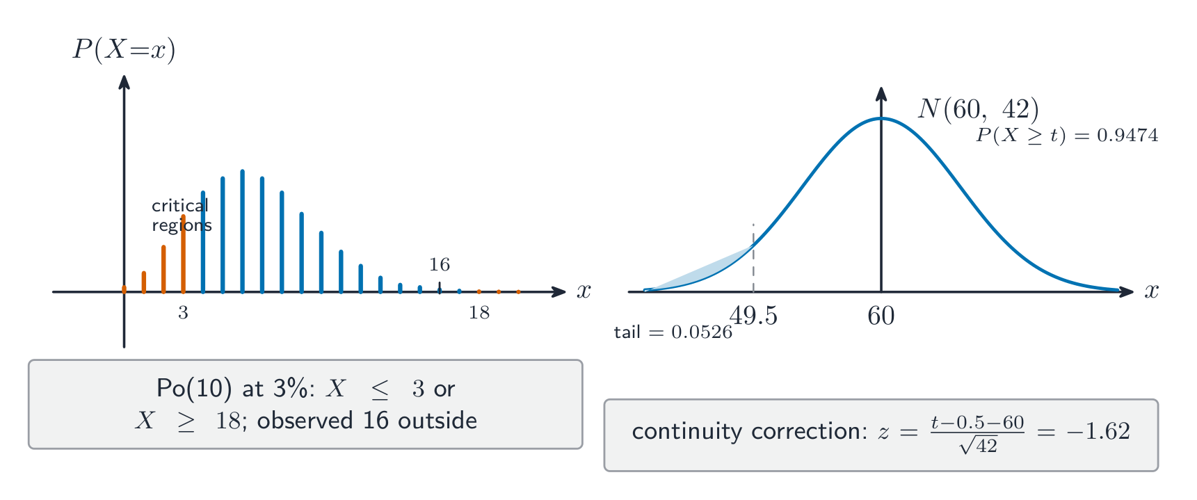
Worked example — a Poisson rate test (WST02 June 2025 Q2). Customers average 20/hour;
after alterations one 30-minute interval is watched: $X\sim\mathrm{Po}(10)$, $H_0\colon\lambda = 10$,
$H_1\colon\lambda \ne 10$. At 3%: $P(X \le 3) = 0.0103$ but $P(X \le 4) = 0.0293$ (too big);
$P(X \ge 17) = 0.0270$ but $P(X \ge 18) = 0.0143$ — critical region $X \le 3$ or $X \ge 18$,
actual level $0.0103 + 0.0143 = 2.46\%$. The observed 16 lies outside → do not reject $H_0$.
Worked example — binomial test with a Normal middle (WST02 June 2025 Q7). 30% of
customers take insurance; a sample of 40 gives $X\sim B(40, 0.3)$. Largest $r$ with
$P(X < r) < 0.05$ (fewer than $r$): $P(X \le 6) = 0.0238 < 0.05$ but $P(X \le 7) =
0.0553 > 0.05$, so $r = 7$. For 200
customers, $B(200, 0.3)\approx N(60, 42)$: $P(X \ge t) = 0.9474$ means
$\tfrac{t - 0.5 - 60}{\sqrt{42}} = -1.62$, so $t = 50$. After a special offer, 11 of 25 buy:
$H_0\colon p = 0.3$, $H_1\colon p > 0.3$; $P(X \ge 11) = 0.0978 < 0.10$, so reject $H_0$ —
evidence the proportion has increased.
Checklist before you call this unit done
State binomial/Poisson assumptions in context; solve mean/variance pairs for $n$, $p$; scale Poisson rates with time.
Normalise piecewise densities (constants, perfect-square k); differentiate F for f; find median/quartiles from F, mode from f' or corners; run E(X), E(X²), Var; read skewness from mean–median–mode.
Quote and derive the uniform facts; pin a and b from an interval plus the mean; keep probabilities as lengths.
Distinguish census vs sample with pros and cons; recognise statistics; build small sampling distributions by enumeration; wrap counts in B(n, p) for follow-ups.
Run one- and two-tailed tests: hypotheses in symbols and words, critical region by accumulation, actual significance level, in-context conclusion; Normal approximation with continuity correction when n is large.
Decision Mathematics 1: algorithms, networks and linear programming
English
Decision Mathematics 1 (D1, paper WDM01/01, 1 hour 30 minutes, 75 marks, first assessment
June 2019) is the discrete option of the IAL: P1–P2 are assumed, and every method is an
ALGORITHM — a finite list of exact instructions. No formula booklet entries beyond the
basics: the marks are for executing procedures precisely and stating results in the required
form. This reference covers sorting and packing algorithms, minimum spanning trees,
shortest paths, the Chinese postman and travelling salesman problems, critical path
analysis and linear programming.
House rules for algorithm answers:
Task
Required form
sorting
list the list after EACH pass (or pivot choices for quick sort)
bin packing
name the algorithm (first-fit, first-fit decreasing, full-bin) and show each placement
graph algorithms
state the order edges/nodes are chosen; show final values (labels, total weight)
route inspection
list the odd nodes, the pairings and their weights, before totalling
linear programming
define variables, objective and EVERY constraint with non-negativity
The bubble sort 冒泡排序 compares adjacent items, swapping out-of-order pairs, one pass
at a time; a pass with no swaps ends it. The quick sort 快速排序 picks the MIDDLE item
of the list as pivot, partitions the remaining items into "less than pivot" and "greater
than pivot" sublists (keeping their order) and recurses — always quote the pivot and the
list after each partition. The spec pins the middle-item choice to the method defined in
its glossary, so exercise lists here keep an odd number of items and the middle item is the
one at position $\tfrac{n+1}2$. Bin packing 装箱问题: first-fit places each item in the
first bin with room; first-fit decreasing sorts items largest-first then applies
first-fit; full-bin packing looks for combinations filling a bin exactly.
A minimum spanning tree (MST) 最小生成树 connects every vertex at least total weight.
Kruskal's algorithm 克鲁斯卡尔算法: sort edges by weight, add the smallest that does
NOT form a cycle (reject and move on when it would). Prim's algorithm 普里姆算法: grow
a tree from any start vertex, repeatedly adding the cheapest edge from the tree to a new
vertex. The matrix form of Prim: cross out the start row, ring the cheapest remaining entry
in the column of the chosen vertex, and continue. Kruskal is edge-driven (good on a drawn
network); Prim is vertex-driven (good on a matrix). Both give the same total; edges may
differ only when weights tie.
Worked example (original). Edges AB 4, AC 2, BC 3, BD 5, CD 1: Kruskal takes CD 1,
AC 2, BC 3 (B joins — no cycle), then rejects AB 4 and BD 5 (cycles): MST total 6. Prim
from A: AC 2, CD 1 (cheapest edge from {A,C} to a new vertex), CB 3: the same tree, and
the total 6 ✓. Always list the edges in the order chosen and give the total.
Dijkstra's algorithm 迪杰斯特拉算法 labels vertices with the smallest total distance
found so far: start vertex label 0; repeatedly pick the unlabelled vertex of smallest
temporary label, make it permanent, and update its neighbours
(new = permanent + weight, only if smaller). Record the order of permanence and the final
labels; the route is recovered by tracing back through vertices whose label equals the
final label minus the connecting weight.
Worked example (original). Edges AB 4, AC 2, BC 1, BD 5, CD 8. Labels: A = 0 permanent;
C = 2 permanent; B = min(4, 2+1) = 3 permanent; D = min(3+5, 2+8) = 8 permanent. The
shortest route from A to D has length 8: A–C–B–D (trace back: 8 = 3 + 5 at B, 3 = 2 + 1 at
C).
The route inspection (Chinese postman) problem 中国邮递员问题 walks every EDGE at least
once and returns to the start. Total length = total of all edges + the shortest way to
duplicate edges so every vertex becomes even. Find the odd vertices (at most four), list
their pairings, choose the pairing of least total weight, and duplicate those edges. State
the pairing before the total.
Worked example (original). Edges AB 4, AC 2, BC 3, BD 5, CD 1 (total 15). Degrees: A 2,
B 3, C 3, D 2 — the odd nodes are B and C, so duplicate BC (weight 3): the shortest closed
route walking every edge at least once has length 15 + 3 = 18.
The classical travelling salesman problem 旅行商问题 tours every VERTEX exactly once
and returns, on a complete graph with the triangle inequality. Bounds: a lower bound is the
MST of the network doubled is an UPPER bound route (walk each MST edge twice); a better
upper bound applies shortcuts. Lower bounds come from MST-based arguments (e.g. the MST
itself, or deleting a vertex and adding its two cheapest edges). The nearest neighbour
algorithm 最近邻算法 builds a tour: from the start vertex repeatedly go to the nearest
unvisited vertex, then return. Convert to a complete network of shortest distances first
when the graph is not complete (via Dijkstra or inspection).
Worked example (original). Complete network: AB 4, AC 2, AD 7, BC 3, BD 5, CD 6 (the
triangle inequality holds throughout). Nearest neighbour from A: A–C (2), C–B (3), B–D (5),
D–A (7): tour length 17 — an upper bound. The MST is AC + BC + BD = 10, so doubling it
gives the crude upper bound 20, improved to 17 by shortcuts; a lower bound from deleting A
(MST of B, C, D is 3 + 5 = 8, plus A's two cheapest edges AC + AB = 2 + 4 = 6) is 14. The
optimal tour lies between 14 and 17.
Model a project as an activity-on-arc network 活动在弧上的网络 from a precedence table;
dummies 虚活动 (zero-weight arcs) resolve dependencies that shared endpoints cannot
express. The critical path 关键路径 is the longest chain through the network: the
project duration. Compute earliest event times 最早事件时间 (forward pass: the max of
arrivals) and latest event times 最晚事件时间 (backward pass: the min of departures).
An activity's total float 总时差 = latest finish − earliest start − duration; critical
activities have zero float. Gantt (cascade) charts 甘特图 bar each activity from its
earliest start with its float as a trailing space; scheduling allocates workers day by day.
Worked example (original). Activities A (3 days), B (4), C (4 after A), D (1 after B),
E (5 after C and D). Chain A–C–E = 12 days; chain B–D–E = 10 days: the critical path is
A–C–E and the project takes 12 days; D's total float = 12 − (4 + 1 + 5) = 2 days.
Formulate: define the decision variables, write the objective (maximise/minimise) and every
constraint as an inequality, including $x, y \ge 0$. Solve two-variable problems graphically:
shade the feasible region, then use the ruler method 尺子法 (slide a ruler along the
objective's gradient) or the vertex method 顶点法 (evaluate the objective at each vertex
of the feasible region). Integer solutions: test integer points near the optimal vertex
inside the region.
Execute bubble and quick sorts showing every pass and pivot; bin pack by first-fit, first-fit decreasing and full-bin with placements shown.
Find MSTs by Kruskal and by Prim (node and matrix forms); draw a network from a matrix and back.
Run Dijkstra with labels in order of permanence; recover the route, not just the length.
Solve route inspection: odd nodes, all pairings with weights, least duplication, total walk length.
Bound the classical TSP: doubled MST and shortcuts for upper bounds, MST-deletion for lower bounds; run nearest neighbour on the complete shortest-distance network.
Build activity networks with dummies; forward and backward passes for event times; total floats; identify the critical path; draw the Gantt chart and schedule.
Worked example (original). Activities A (3 days), B (4), C (4 after A), D (1 after B),
E (5 after C and D). Chain A–C–E = 12 days; chain B–D–E = 10 days: the critical path is
A–C–E and the project takes 12 days; D's total float = 12 − (4 + 1 + 5) = 2 days.
Worked example — linear programming (original). Maximise $P = 3x + 2y$ subject to
$x + y \le 10$, $2x + y \le 14$, $x, y \ge 0$. The feasible region's vertices are
$(0,0)$, $(7,0)$, $(4,6)$, $(0,10)$; evaluating $P$: 0, 21, 24, 20 — the maximum is
$P = 24$ at $(4,6)$, where both constraints are tight.
Formulate linear programs fully; solve graphically by ruler or vertex methods; find best integer solutions.


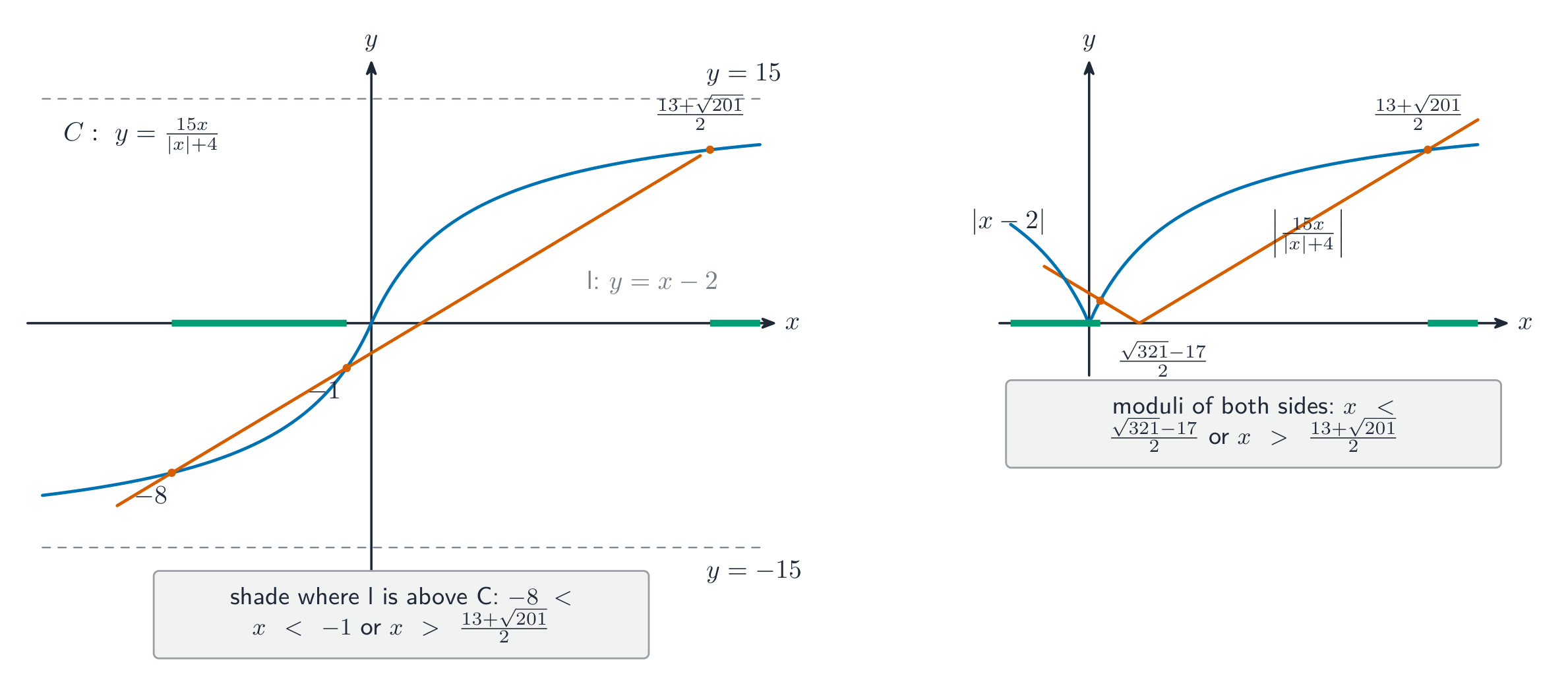
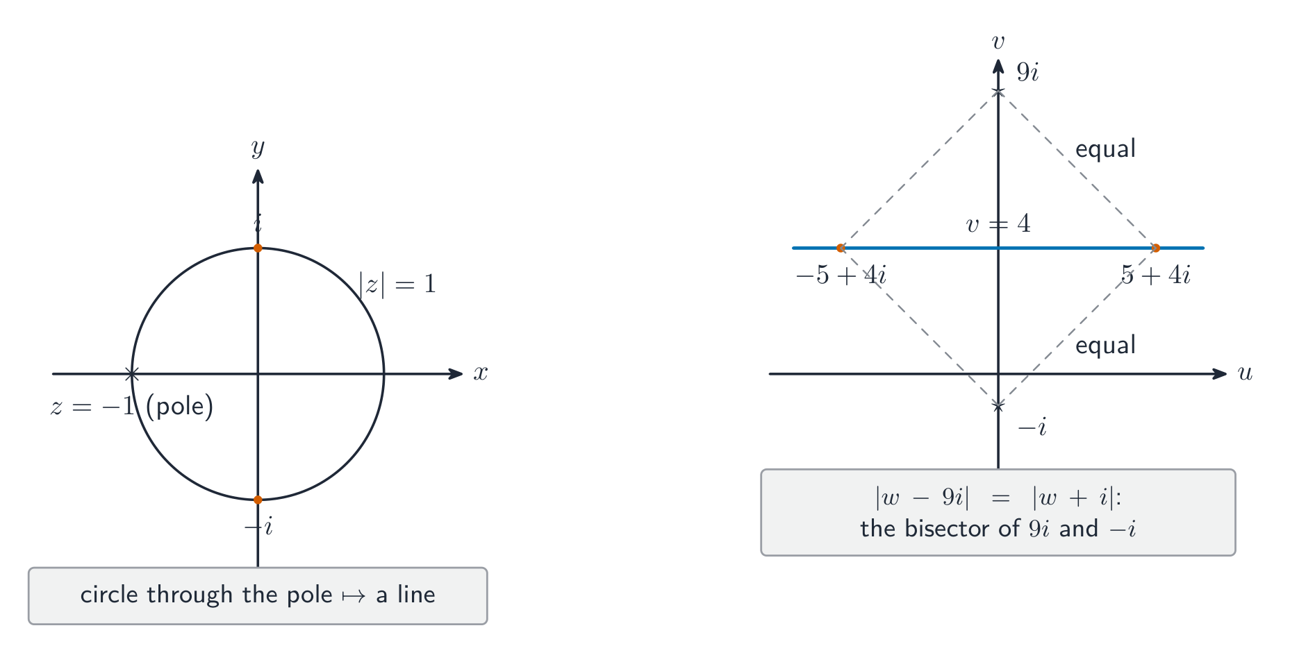
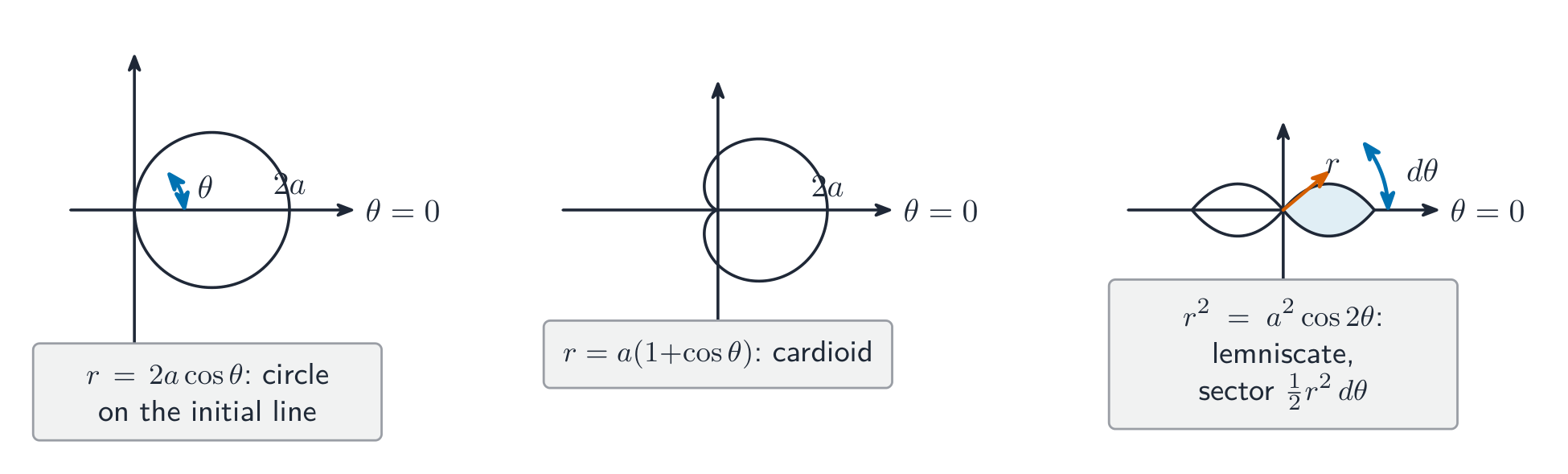


![Left: the CDF F(x) = (6x^2 - x^4)/5 on [0, 1] rising from 0 to 1 with the median marked at F = 1/2 (x = 0.671). Right: the density f(x) = (12x - 4x^3)/5 with the mode at x = 1 and the area beyond x = 0.6 shaded (0.594).](/handout-media/edexcel_ial_further_mathematics/assets/08-cdf-pdf.png?v=1792133600)
![Left: a triangular pdf rising along 2x/21 from 0 to k = 3.5 then falling along 2(6-x)/15 to x = 6, peak value 1/3 marked. Right: the uniform density on [-2, 14] at height 1/16 with the interval [8, 14] shaded (area 3/8).](/handout-media/edexcel_ial_further_mathematics/assets/08-triangular-pdf.png?v=1792133600)