Uncertainty, gradients and model testing
Introduced| English | Meaning |
|---|---|
| systematic error/ˌsɪstəˈmætɪk ˈerə/ | A consistent measurement bias caused by the method or instrument. |
| uncertainty/ʌnˈsɜːtənti/ | An estimate of the possible range of error in a measurement. |
What would explain this observation?
- A line passing near every data point is useful, but its gradient can still be uncertain. A graph is evidence for a model within the measurement range.
Build the model
- Random variation makes repeated readings differ.
- Systematic error 系统误差 shifts results consistently.
- Absolute uncertainty 不确定度 has the measured unit; relative or percentage uncertainty compares uncertainty with the measured value.
- uncertainty: A quantified limitation on a measured result.
- systematic error: A consistent measurement bias.

Which is most likely a systematic error?
Difficulty 1/5 · 100 coins + a small bonus on first completion today
A fixed 0.20 g balance zero offset is a systematic error. Independent repeats reduce random uncertainty in the mean, not scatter in individual readings or a shared offset. Reaction timing can have both random and systematic contributions.
Match each technical term to its precise meaning.
Difficulty 2/5 · 140 coins + a small bonus on first completion today
Use the definitions to distinguish related quantities and processes.
Choose evidence that can test it
- For a product or quotient, adding fractional uncertainties is a common maximum-uncertainty approximation.
- For a difference, add absolute uncertainties.
- A nonzero intercept can reveal an offset or an incomplete model.
In the lab: Show units on axes and choose a sensible scale. Plot uncertainty bars where justified, draw a best-fit line rather than joining every point, and estimate steepest and shallowest plausible gradients when the course method calls for them.
Which two habits make the investigation or model in this case more defensible?
Difficulty 2/5 · 140 coins + a small bonus on first completion today
Stating the conditions and assumptions lets others repeat the work exactly, and recording the supporting evidence lets them check the conclusion. Hiding disagreeing results removes the evidence that could challenge a wrong conclusion, and one measurement can never establish a wider claim.
Work from known quantities
- Known: length = 50.0 mm with uncertainty 1.0 mm.
- Percentage uncertainty = absolute uncertainty/value ×100 = 1.0/50.0×100 = 2.0%.
- For a quotient of two independently measured quantities with maximum percentage uncertainties 2% and 3%, the summed maximum estimate is 5%.
Your turn: A 40 cm reading has an absolute uncertainty of 1 cm. Find percentage uncertainty.
Measurement ranges and the quotient estimate
50 ± 1 mm has a 2% uncertainty. Compare it with a 100 ± 3 mm reading: the summed quotient estimate is 5%, while exact endpoint calculations reveal a slightly asymmetric range.
A 40 cm reading has an absolute uncertainty of 1 cm. Find percentage uncertainty.
Difficulty 2/5 · 140 coins + a small bonus on first completion today
The result is 2.5 %. Known: reading 40 cm; absolute uncertainty 1 cm. Use percentage uncertainty = absolute uncertainty / value x 100. Percentage uncertainty = 1/40 x 100 = 2.5%. Smaller measured values carry larger percentage uncertainties for the same absolute uncertainty.
Check the conclusion and its limits
- Repeating readings reduces random uncertainty in a mean but does not automatically remove a zero error.
- Do not quote more decimal places than your measurement can support.
Not true: Repeating a measurement always removes a calibration offset. Independent repeats and averaging can reduce random uncertainty of the mean, while a calibration offset can remain. Check calibration and apply a justified correction where appropriate.
- Random variation makes repeated readings differ.
- For a product or quotient, adding fractional uncertainties is a common maximum-uncertainty approximation.
- Watch for: repeating readings reduces random uncertainty in a mean but does not automatically remove a zero error.
Repeating a measurement always removes a calibration offset.
Difficulty 1/5 · 100 coins + a small bonus on first completion today
Independent repeats and averaging can reduce random uncertainty of the mean, while a calibration offset can remain. Check calibration and apply a justified correction where appropriate.
A quantified limitation on a measured result: write the technical term.
Difficulty 1/5 · 100 coins + a small bonus on first completion today
uncertainty means A quantified limitation on a measured result.
Write from the data: find the uncertainty
- A 40 mm reading has an absolute uncertainty of 6 mm.
- Find the percentage uncertainty. For a quotient, add the percentage uncertainties.
A 40 mm reading has an absolute uncertainty of 6 mm. What is the percentage uncertainty, and how are two percentage uncertainties combined for a quotient?
6 divided by 40 is 0.15, which is 15 percent. Adding percentages is the maximum-uncertainty rule used here.
The HL written reading is 40 mm with absolute uncertainty 6 mm. Find percentage uncertainty and state the taught quotient-bound convention.
Difficulty 1/5 · 100 coins + a small bonus on first completion today
Percentage uncertainty = absolute uncertainty/reading × 100 = 6/40 × 100 = 15%. For a quotient, add the two percentage uncertainties under the taught first-order maximum-bound approximation; this is not a confidence interval.
Turn a biological explanation into a measurable comparison
- A useful question specifies organism, treatment range, measured response and interval. Instead of asking whether plants like light, investigate how daily light duration affects change in a stated seedling's shoot length over seven days. Explain why photosynthetic supply might affect growth while other limits can change the response.
- A hypothesis proposes an explanation; a prediction states what observations should follow under defined conditions. Experiments assign a treatment, while surveys examine observed differences. A database or simulation can support inquiry too, but selection rules, origins and assumptions must be explicit. Correlation between shade and density does not exclude soil moisture or disturbance as alternative causes.
Identify the independently assigned experimental unit
- If a whole tray receives a light-duration treatment, seedlings within that tray are subsamples. Four seedlings measured on five days do not provide twenty independent treatment replicates. Use several independently assigned trays per treatment where feasible and analyse variation at the level justified by the design.
- Repeated readings can describe time or reading repeatability without adding independent organisms or trays. The figure uses three trays per treatment and four seedlings per tray as a model, not a compulsory sample size. Independent replication estimates variation among treatment units; more treatment levels instead help reveal response-curve shape.
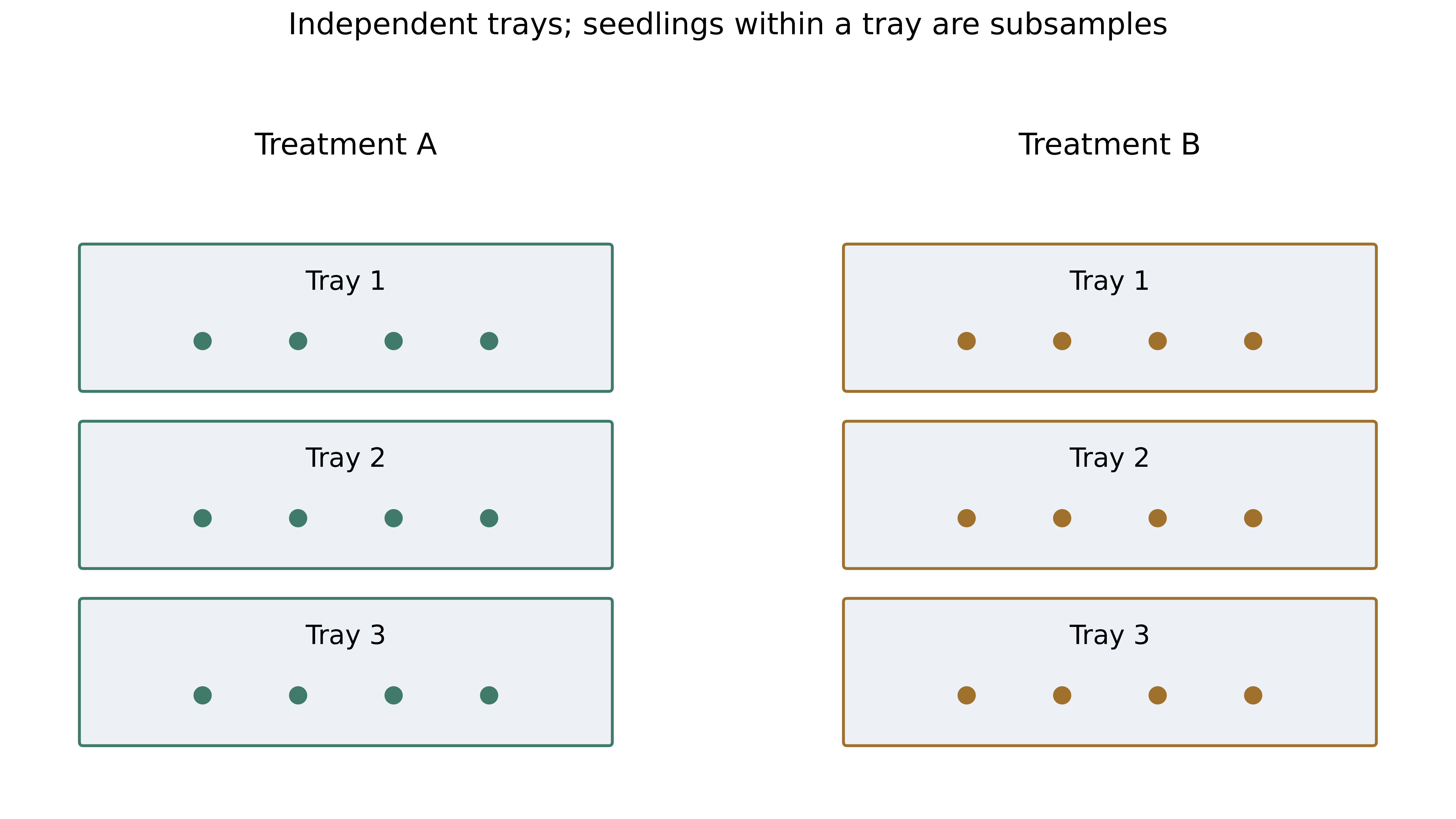
Each light duration is assigned to one whole tray, with four seedlings measured on five days. Which statement correctly identifies replication?
Difficulty 1/5 · 100 coins + a small bonus on first completion today
Experimental units follow independent assignment, not the number of rows in the dataset. Subsampling and repeated readings have useful but different roles.
Connect controls, randomization and a pilot with the main comparison
- Random treatment assignment reduces systematic allocation differences; random sampling helps represent a population. Blocking can group similar bench positions, with treatments randomized within each block. Controlled variables such as age, water and soil need a stated method and biological reason, rather than a list claiming everything remained constant.
- A control treatment supplies a comparison. Solvent-only controls help separate a substance from its carrier, while a positive control can show a detector responds to a known signal. Pilot the range, safety, timing and resolution before main collection. Neither randomization nor a pilot automatically repairs a tiny sample or a confounded design.
Preserve a safe, ethical and reproducible record
- Identify the hazard, possible exposure and a specific control: for example, cutting tools, heat or electricity near liquid. Obtain teacher approval for actual work. Do not culture unknown environmental microbes or impose harmful treatments on people or animals. Field work needs appropriate permission and habitat protection; human observations require consent, privacy and withdrawal.
- Record dates, source organisms, assignments, calibration, timings, settings and deviations as they occur. Preserve original raw data separately from calculations, including failed readings and documented causes. Credit data, methods, images and code. Do not invent missing observations or release laboratory organisms; shared collection does not make another person's analysis or final report your own.
Separate accuracy, precision and validity
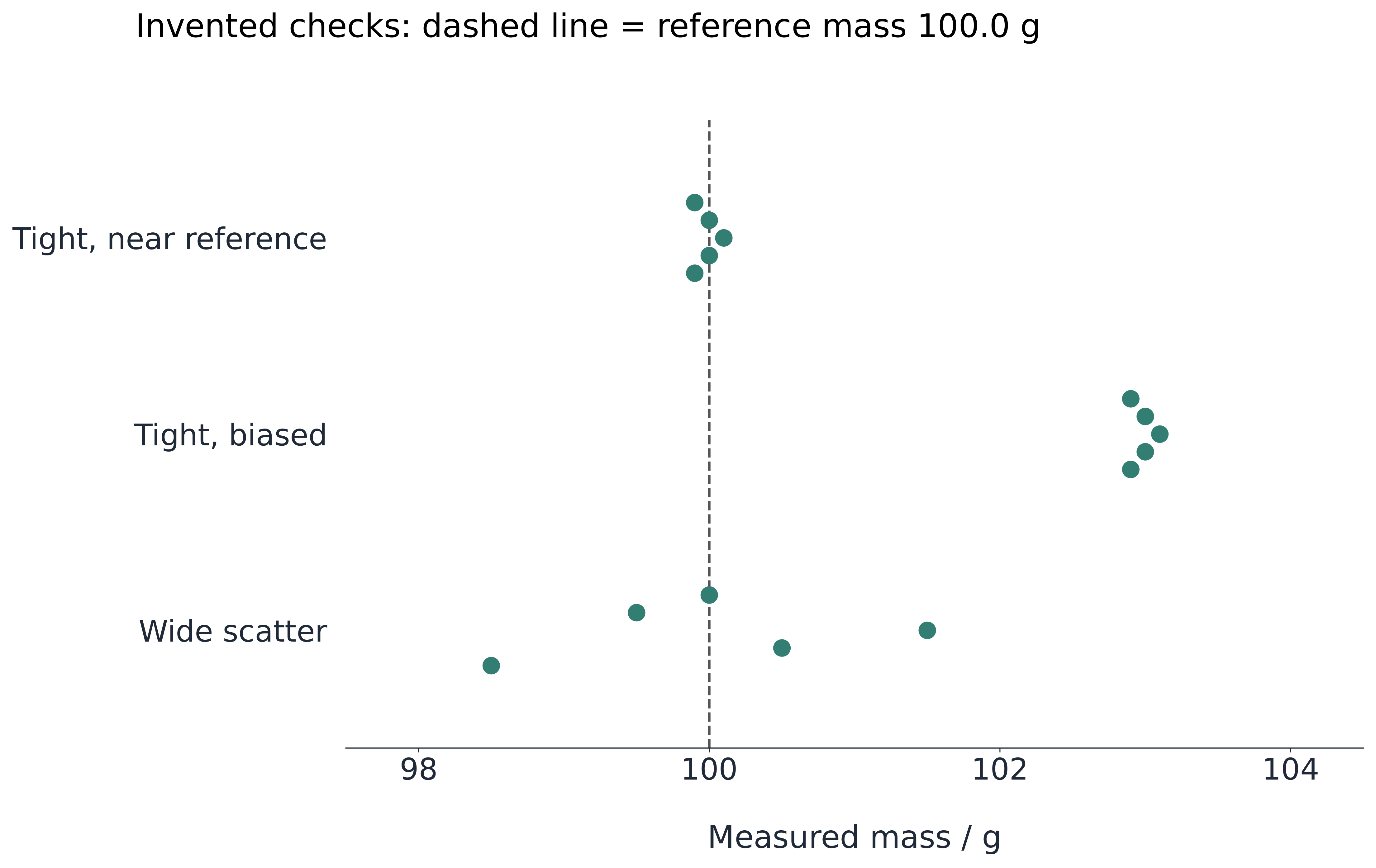
- Accuracy concerns agreement with a suitable reference; precision concerns closeness among repeats. A tightly clustered set 0.8 g above a reference is precise but biased. Validity asks whether the method supports the question and interpretation: repeating a confounded design consistently does not make its causal conclusion valid.
- Check tare, relevant standards and calibration range. A zero offset can shift all readings, while a scale-factor error can distort a calibration slope. Independent averaging may reduce random uncertainty in a mean but retains uncorrected bias. Check the cause and apply a justified correction or improve calibration; one successful reference check does not validate all values and conditions.
State what an uncertainty estimate represents
- Uncertainty can reflect resolution, repeat scatter, calibration or a supplied maximum bound. Absolute uncertainty has the quantity's unit; percentage uncertainty compares it with the measured value. For 50.0 ± 1.0 mm, the percentage is 2.0%; for 40 ± 1 cm, it is 2.5%, despite the same numerical uncertainty of one.
- Half an analogue division can be a simple reading estimate, but is not a universal rule. A digital last digit does not include every calibration or method contribution. Distinguish stated maximum bounds from standard uncertainties or confidence intervals, and consider dependence between measurements before propagating them.
Use an image scale that remains connected to the measured object
- Begin microscopy at low power, using suitable thin specimens and approved stains where appropriate. Draw observed structures with clear outlines, labels and a scale; separate observation from inferred identity. Calibrate an eyepiece graticule with a stage micrometer for the objective used, rather than transferring one calibration to every objective.
- In an invented image, a 20 mm bar represents 50 micrometres. A 32 mm cell on the same copy is 80 micrometres; magnification is 20/0.050 = 400, a unitless ratio. Resizing image and bar together preserves the cell-to-bar ratio, but changes printed magnification. Always convert image and actual lengths to matching units before dividing.
An invented micrograph has a 25 mm image bar representing 100 micrometres. A cell is 15 mm on the same image copy. Find actual cell length in micrometres.
Difficulty 2/5 · 140 coins + a small bonus on first completion today
15/25 × 100 = 60 micrometres. The cell-to-bar ratio survives resizing when both scale together; printed magnification does not remain fixed.
Interpret chromatography as conditional separation evidence
- Mark an origin above the solvent and apply a suitable spot without dissolving it directly into the reservoir. Components separate through different interactions with the mobile and stationary materials. Mark the solvent front promptly. Both distances for Rf start at the origin, not the paper edge.
- A pigment travelling 36 mm while the front travels 60 mm has Rf = 0.60, with no unit. The separate 42/70 case also gives 0.60. A matching reference under identical conditions supports identification, but similar movement alone is not unique chemical proof. Solvent, material and handling differences can change separation.
Use calibration and cumulative dilution with their stated ranges
- Colorimetry needs an appropriate blank, consistent cuvettes/path length and standards. For invented calibration A = 0.20c + 0.04, with c in mg/L and A dimensionless, A = 0.44 gives c = 2.0 mg/L. Interpolate within the validated range; turbidity, saturation or a different sample matrix can invalidate the relation.
- Transfer 1.0 mL stock into 9.0 mL diluent and mix: final volume is 10.0 mL, a tenfold dilution. Three successive steps take 2.0 mg/mL to 0.0020 mg/mL. Retain the cumulative factor when recovering the original concentration and use suitable clean equipment; another transfer from an unmixed layer need not have the intended concentration.
An invented validated calibration is A = 0.20c + 0.04, where c is mg/L and absorbance A is dimensionless. An unknown within the calibrated range has A = 0.64. Find c.
Difficulty 2/5 · 140 coins + a small bonus on first completion today
c = (0.64 − 0.04)/0.20 = 3.0 mg/L. Subtract the intercept and respect blank, matrix and calibration-range conditions.
An invented 5.0 mg/mL stock undergoes three successive tenfold dilutions, mixing each time. Find the final concentration.
Difficulty 2/5 · 140 coins + a small bonus on first completion today
5.0/10³ = 0.0050 mg/mL. Each transfer is a further tenfold step; retain the cumulative factor and distinguish aliquot volume from final volume.
Make field and digital selection rules reproducible
- Preselect quadrat positions using a justified random or stratified design; use a transect for a defined gradient. Record area, boundary rules and identification method, using keys with contrasting observable characters. Karyograms compare chromosomes, cladograms infer relationships, and molecular models represent selected features; one picture does not directly measure every feature it suggests.
- Sensors need recorded frequency, drift and response delay. Image analysis needs calibration, segmentation rules and example checks; overlapping objects may merge. Match database units, dates, definitions, effort and missing-data rules. Save spreadsheet formulas/settings and independently check rows. Changing a simulation parameter tests its model, not automatically a real ecosystem.
Separate sample scatter from uncertainty in a mean
- Invented independent rates 4, 5, 5, 6 and 10 mm per day have mean 6, median 5 and range 6. Squared deviations sum to 22; sample SD is about 2.35 mm per day and SE about 1.05 under the independence model. SD describes scatter among measurements, while SE concerns the estimated mean; neither equals the instrument resolution by definition.
- Excluding the central value for the stated quartile convention gives lower-half median 4.5 and upper-half median 8, so IQR is 3.5. Other software conventions can differ. Investigate the value 10 without deleting a valid inconvenient observation. Preserve raw replicates and document justified exclusions and their consequences.
Invented independent rates are 2, 3, 3, 4 and 8 mm per day. Their mean is 4 and squared deviations sum to 22. Find the sample standard deviation.
Difficulty 2/5 · 140 coins + a small bonus on first completion today
Sample SD = √[22/(5 − 1)] = √5.5 ≈ 2.35 mm per day. SD concerns scatter, not the uncertainty of the estimated mean.
For five independent invented rates with sample SD √5.5 mm per day, calculate the standard error of the mean.
Difficulty 2/5 · 140 coins + a small bonus on first completion today
SE = √5.5/√5 = √1.1 ≈ 1.05 mm per day under the independence model. Repeated observations from one unit are not automatically five independent units.
Propagate the specified bounds rather than inventing a confidence interval
- For readings 12.0 ± 0.1 g and 10.0 ± 0.1 g, the difference is 2.0 ± 0.2 g using summed absolute maximum bounds. A rate from change 6.0 ± 0.4 mm over 3.0 ± 0.1 days is 2.0 mm per day; summing fractional bounds gives 0.4/6.0 + 0.1/3.0 = 0.10, an approximate maximum uncertainty of 0.2 mm per day.
- This first-order product/quotient convention differs from quadrature of independent standard uncertainties and from a statistical confidence interval. Dependence and uncertainty definitions matter. Give units and justified precision, state the convention, and avoid claiming that repeated measurements automatically remove a shared calibration offset.
An invented change is 8.0 ± 0.4 mm over 4.0 ± 0.2 days. Using summed fractional maximum bounds, estimate the absolute uncertainty of the calculated rate.
Difficulty 2/5 · 140 coins + a small bonus on first completion today
Rate = change/time = 8.0/4.0 = 2.0 mm per day. Fractional maximum-bound estimate = 0.4/8.0 + 0.2/4.0 = 0.05 + 0.05 = 0.10. Absolute rate uncertainty ≈ 2.0 × 0.10 = 0.20 mm per day. This first-order convention is not a statistical confidence interval or an automatic quadrature rule.
Interpret graph gradients and intercepts using the biological model
- Use a scatter graph for two quantitative variables, bars for categories and a histogram for a continuous distribution; unequal histogram widths require frequency density when area represents frequency. Label all error bars and give sample size. A high R² does not make the association causal or state the fraction biologically caused by the predictor.
- In the invented length series 10, 12, 14 and 16 mm at days 0, 1, 2 and 3, gradient is 2.0 mm per day and intercept 10 mm is starting length. With ±0.5 mm length bounds and exact time, shallow and steep endpoint lines give 5/3 and 7/3 mm per day, both also crossing the middle bounds here. Their envelope is about 2.00 ± 0.33 mm per day, not a regression confidence interval. A nonzero intercept need not be an error; on a curve, a tangent and a chord answer different rate questions.
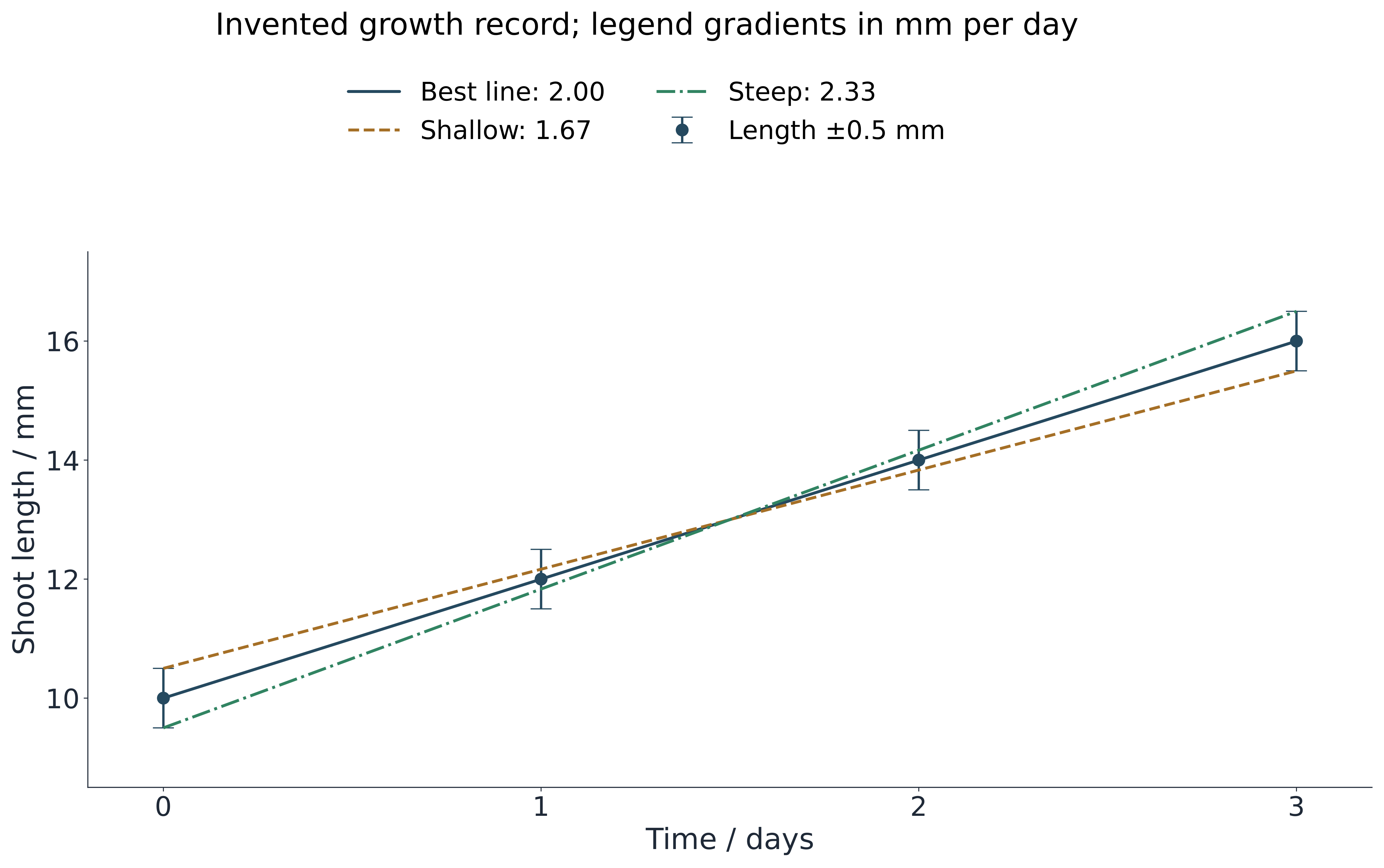
An invented best-fit line goes through length 10 mm at day 0 and 16 mm at day 3. Find its gradient.
Difficulty 2/5 · 140 coins + a small bonus on first completion today
(16 − 10)/(3 − 0) = 2 mm per day. The intercept represents starting length in this model; forcing the line through zero would change the question.
Match a statistical test to the question and sampling design
- Pearson correlation assesses a linear association, so near-zero correlation can hide a curved pattern. A suitable t-test compares means under its independent or paired design and distribution/variance assumptions. Chi-squared concerns suitable category counts with adequate expected counts and appropriate independence. Repeated readings are not independent organisms merely because a test needs a larger sample.
- At a preselected 0.05 level, an invented valid test with p = 0.03 supplies evidence against its null model, while p = 0.12 does not reach that threshold. A p-value is not the probability the hypothesis is true or that chance caused the observation. Non-significance does not prove zero effect; report effect size, variation, sample size, assumptions and biological importance too.
Name the ecological estimator and its assumptions
- With 40 animals initially marked, 50 caught later and ten marked recaptures, the Lincoln estimate is 40 × 50/10 = 200. It requires suitable closure, retained marks, mixing and comparable capture; it is not a census. Changing recapture probability can bias the answer even if the arithmetic is correct.
- For species counts four and six, Simpson's reciprocal finite-sample form N(N − 1) divided by the sum of n(n − 1) gives 90/42, about 2.14. The alternative reciprocal of summed squared proportions gives about 1.92 for these same data. State the formula rather than mixing them; neither result means 2.14 or 1.92 species were observed. Appropriate sampling and consistent definitions precede calculation.
Two species have invented counts five and five. Use the stated reciprocal finite-sample form N(N − 1)/Σ[n(n − 1)] to calculate Simpson’s index.
Difficulty 2/5 · 140 coins + a small bonus on first completion today
N = 10; 10 × 9/[5 × 4 + 5 × 4] = 90/40 = 2.25. State the formula: another convention gives a different small-sample value, and only two species were observed.
Close the chain from a measured effect to a qualified conclusion
- Answer the actual question with the observed direction, size, range and uncertainty, explaining relevant biology and alternatives. Then connect a specific limitation to its likely consequence and feasible improvement: an unresolved 0.4 mm change with ±0.5 mm readings calls for a suitably calibrated method, while shared tray treatments call for more independent trays, not more readings of the same roots.
- Preserve authentic records, formulas, exceptions and credited sources. Supervised practical work develops skills that a lesson cannot replace. Individual investigation needs independent reasoning/authorship, while collaborative science develops joint inquiry and communication. Evaluation should prioritize limitations that can change the conclusion, rather than list disconnected generic mistakes or promise a guaranteed assessment result.
Design a teacher-approved low-risk biological comparison, then explain how raw records, uncertainty, statistical decisions and evaluation support its conclusion. Distinguish independent units from repeated measurements.
A defensible conclusion is traceable from question through design and raw evidence to the analysis and its limits.