Sampling populations without choosing the answer
Introduced| English | Meaning |
|---|---|
| population/ˌpɒpjʊˈleɪʃn/ | All the organisms of one species living in a particular area at a particular time. |
| quadrat/ˈkwɒdræt/ | A frame marking a known area used to sample the abundance or distribution of organisms. |
What would explain this observation?
- A field edge looks richer in plants than its centre. Choosing only the richest patches would build the desired result into the sampling method.
Build the model
- A population 种群 consists of organisms of one species in a defined area.
- Random quadrats 样方 estimate density without deliberately selecting patches.
- A transect investigates change along an environmental gradient.
- quadrat: A defined area used for sampling.
- population: Organisms of one species in a defined area.

Which method investigates change from a path into woodland?
Difficulty 1/5 · 100 coins + a small bonus on first completion today
A transect samples at fixed distances along a line, so the change from open path into woodland is recorded systematically. Choosing only large plants or one convenient spot biases the sample and cannot show a gradient.
Match each technical term to its precise meaning.
Difficulty 2/5 · 140 coins + a small bonus on first completion today
Use the definitions to distinguish related quantities and processes.
Choose evidence that can test it
- Estimate total abundance by multiplying mean density by area, with consistent units.
- This assumes sampled areas represent the habitat.
- Patchiness and too few samples widen uncertainty.
In the lab: Choose coordinates with random numbers before visiting the patches. Record quadrat area and counting rules. For a transect, use fixed distances and measure a relevant abiotic variable. Do not damage habitats or sample unsafe locations.
Which two habits make the investigation or model in this case more defensible?
Difficulty 2/5 · 140 coins + a small bonus on first completion today
Stating the conditions and assumptions lets others repeat the work exactly, and recording the supporting evidence lets them check the conclusion. Hiding disagreeing results removes the evidence that could challenge a wrong conclusion, and one measurement can never establish a wider claim.
Work from known quantities
- Known: five 0.25 square metre quadrats contain 3, 4, 6, 5 and 2 plants.
- Mean count = 20/5 = 4.
- Density = 4/0.25 = 16 plants per square metre.
- Estimated abundance in 100 square metres = 16 × 100 = 1,600 plants.
Your turn: Mean count is 6 in a 0.5 square metre quadrat. Find density per square metre.
The estimate depends on which patches you sample
The lesson counts 3, 4, 6, 5 and 2 give a mean of 4 per 0.25 m²: 16 plants/m² and an estimate of 1,600 in 100 m². Compare new random samples with deliberately crowded patches in a known model habitat.
Mean count is 6 in a 0.5 square metre quadrat. Find density per square metre.
Difficulty 2/5 · 140 coins + a small bonus on first completion today
The result is 12 . Known: mean count 6 plants per 0.5 square metre quadrat. Use density = mean count / quadrat area. Density = 6/0.5 = 12 plants per square metre. An abundance estimate scales this density up to the whole area.
Check the conclusion and its limits
- Quadrats suit organisms that do not move quickly.
- A food chain arrow shows the direction of energy transfer, not the direction a predator travels.
Not true: Sampling only the most crowded patches gives an unbiased population estimate. Choosing the most crowded patches overestimates density, because the samples are not representative of the whole area. Unbiased estimation needs random or systematic sampling decided before looking at the plants.
- A population consists of organisms of one species in a defined area.
- Estimate total abundance by multiplying mean density by area, with consistent units.
- Watch for: quadrats suit organisms that do not move quickly.
Sampling only the most crowded patches gives an unbiased population estimate.
Difficulty 1/5 · 100 coins + a small bonus on first completion today
Choosing the most crowded patches overestimates density, because the samples are not representative of the whole area. Unbiased estimation needs random or systematic sampling decided before looking at the plants.
A defined area used for sampling: write the technical term.
Difficulty 1/5 · 100 coins + a small bonus on first completion today
quadrat means A defined area used for sampling.
Write from a density of 20 plants per square metre
- Three quadrats of 0.20 square metres contain 2, 4 and 6 plants.
- Find the mean count and the density. The estimate assumes the quadrats represent the habitat.
Three 0.20 square metre quadrats contain 2, 4 and 6 plants. What are the mean count and the density per square metre?
The three counts sum to 12 and average 4. 4 divided by 0.20 is 20 plants per square metre.
The HL written case gives mean count 4 in a 0.20-square-metre quadrat. Find plants per square metre.
Difficulty 1/5 · 100 coins + a small bonus on first completion today
Mean 4 divided by 0.20 square metres is 20 plants per square metre. Other options — 12 plants per square metre (the earlier calculation's result for a mean of 6 in 0.5 square metres); 16 plants per square metre (the lesson example's result for a mean of 4 in 0.25 square metres).
Define the population before choosing a sample
- A population comprises interacting members of one species in a defined area and period. Specify the target—such as daisies in one lawn this month—rather than mixing all species or leaving the boundary vague. Immigration and emigration can connect neighbouring populations; a survey line is not necessarily a biological wall.
- Generate eligible random coordinates before inspecting abundance. Include sparse and empty places, record inaccessible locations and use one counting rule. Sampling error can remain in a fair sample; bias systematically favours certain results. More repeats improve precision without automatically repairing a biased choice of patches.
Convert quadrat counts through the sampled area
- Quadrats suit rooted or attached organisms. Measure the frame area and define boundary rules; for clonal plants decide whether counts mean shoots or genetically distinct individuals. Cover may be more meaningful when individual organisms cannot be separated reliably.
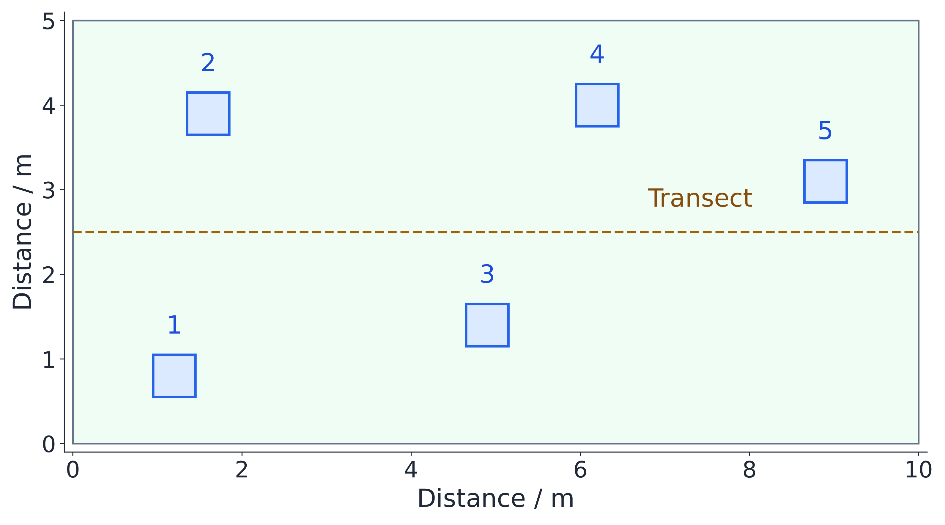
- For invented counts 3, 4, 6, 5 and 2 in five 0.25-square-metre quadrats, mean count is four, density is 16 plants per square metre, and a representative 100-square-metre habitat estimate is 1,600 plants. A transect instead samples change along a chosen gradient; a belt samples a strip. One convenient transect does not automatically represent a whole habitat.
Weight different habitats by their actual areas
- In an invented site, 80 square metres have a representative density of 10 plants per square metre and 20 have density 30. Estimated totals are 800 and 600: 1,400 overall, with area-weighted mean density 14. Simply averaging the densities gives 20 and would overestimate this site.
- Random sampling within defined strata can represent distinct habitats, provided each stratum's estimate uses its actual area. Keep counting, detection and timing comparable. Taking equal numbers of quadrats from unequal areas does not justify giving those areas equal weight in the final whole-site estimate.
An invented survey has an 80-square-metre stratum at 10 plants per square metre and a 20-square-metre stratum at 30. Estimate total abundance.
Difficulty 2/5 · 140 coins + a small bonus on first completion today
80 × 10 + 20 × 30 = 800 + 600 = 1,400 plants. Weight density by actual area; the whole-site mean is 14, not the unweighted mean of 20.
Separate variability among quadrats from uncertainty in a mean
- For counts 3, 4, 6, 5 and 2, sample standard deviation is about 1.58 plants per quadrat. It describes spread among counts. Standard error, under independent-sample assumptions, is about 0.71 plants per quadrat and estimates uncertainty in their mean; neither is automatically a 95% confidence interval.
- Area conversion also applies to these units. Nearby quadrats in one patch may be correlated, exaggerating precision if treated as independent. Three counts 2, 4 and 6 have the same mean as 4, 4 and 4 but different spread; zero observed spread in a small sample does not prove uniformity across the habitat.
Five independent invented quadrat counts have sample standard deviation √2.5 plants per quadrat. Calculate standard error using s/√n.
Difficulty 2/5 · 140 coins + a small bonus on first completion today
√2.5/√5 = √0.5 ≈ 0.707 plants per quadrat, about 0.71. It estimates uncertainty in the mean rather than spread among individual counts, and is not by itself a 95% interval.
Derive mark–recapture from a marked fraction
- Mark M animals in an approved first sample, release and allow mixing, then catch C animals in a second sample, including R marked ones. If that sample represents the population, its marked fraction R/C estimates M/P. Rearranging gives the population estimate below.
- In the invented example, M = 50, C = 60 and R = 15 give an estimate of 200. The second sample is one-quarter marked, suggesting the 50 marked animals form one-quarter of the population. Do not add the two catches or mistake only the recaptured subset for the whole second catch.
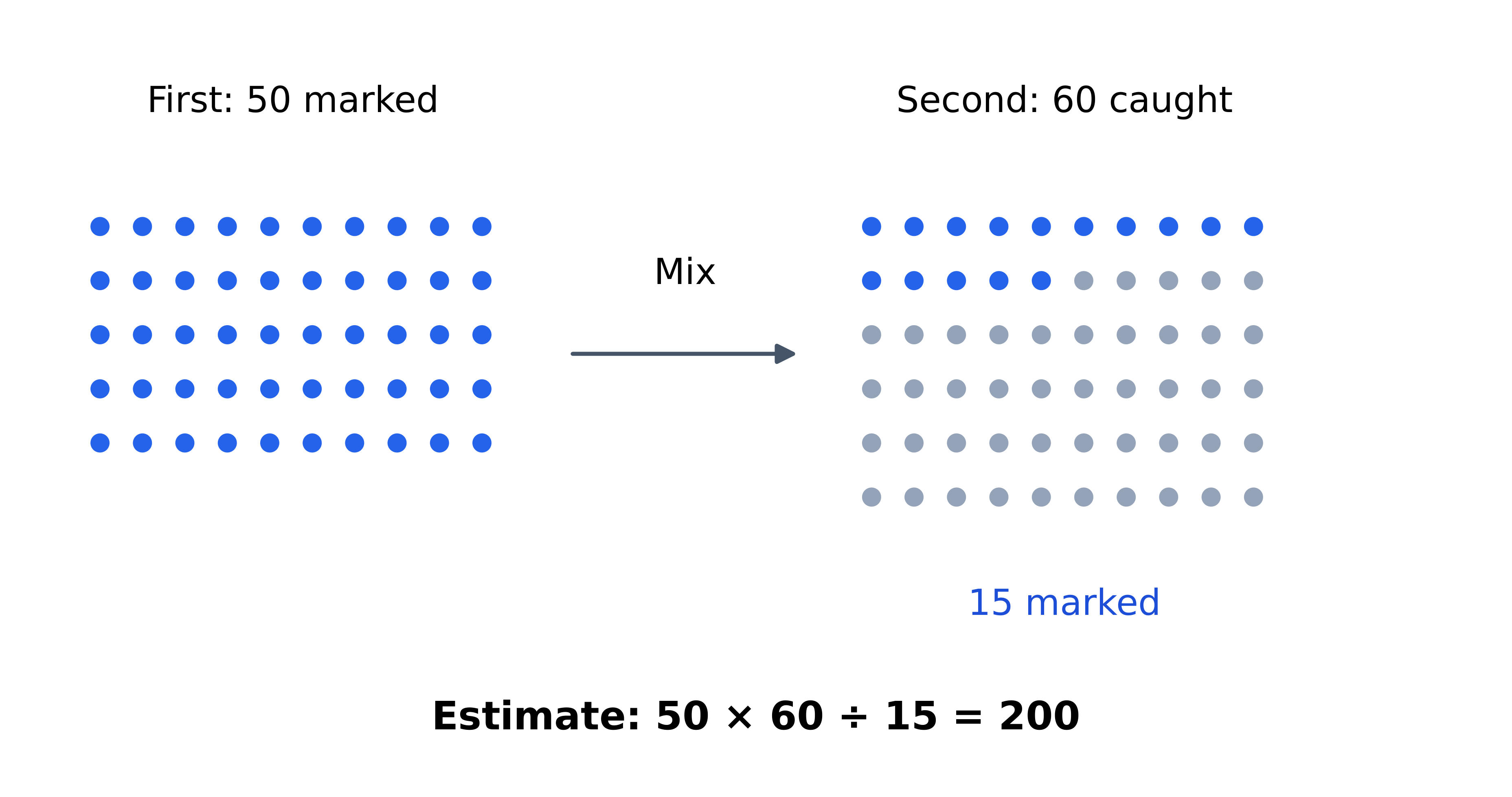
An invented suitable mark–recapture study marks 50 animals, then catches 60, including 15 marked ones. Use M × C / R to estimate population.
Difficulty 2/5 · 140 coins + a small bonus on first completion today
50 × 60 / 15 = 200 animals under the mixing, closure and capture assumptions. The second catch includes both marked and unmarked animals.
Predict the direction of a recapture bias
- The simple model assumes little population change between catches, adequate mixing, retained recognizable marks, and comparable capture probabilities unaffected by marking. Lost marks or trap avoidance can reduce observed recaptures and inflate the estimate; trap attraction can increase recaptures and reduce it.
- Keeping M = 50 and C = 60 but recording R = 12 gives 250 rather than 200, a 25% increase. Very few recaptures make chance especially influential; R = 0 makes the expression undefined, not proof of an infinite population. Use appropriate repeated designs or a better model rather than treating one estimate as exact.
Explain density feedback through gains and losses
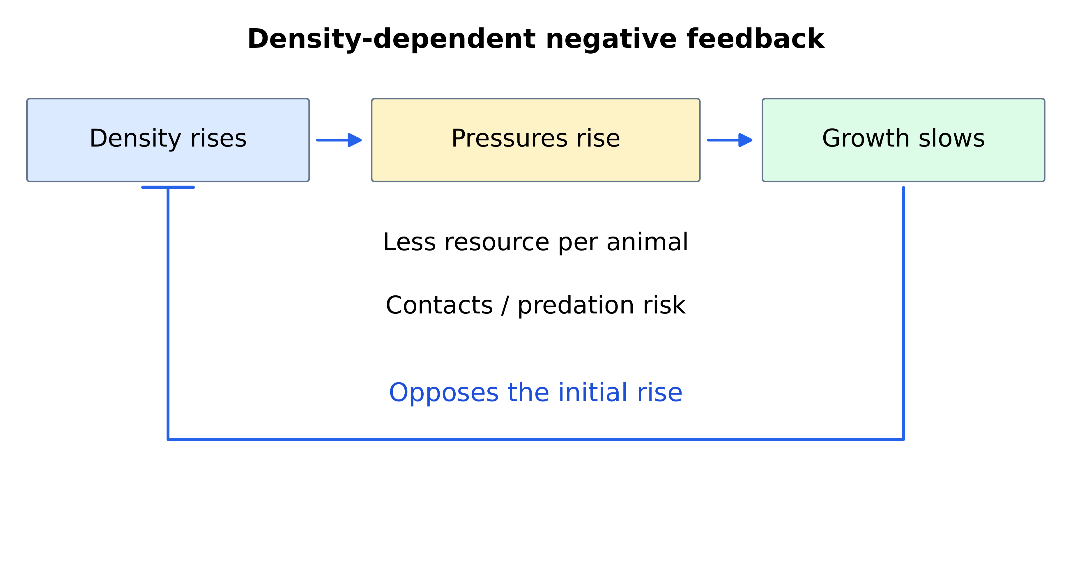
- Carrying capacity is a sustainable population size under stated conditions, rather than a permanent habitat label. Higher density can intensify competition for limiting resources or some forms of disease and predation, reducing per-individual survival or reproduction. Weather and resource changes can also alter the conditions.
- In an invented population starting at 100, 30 births, 10 deaths, four immigrants and six emigrants give net gain 18 and a final 118. At a higher density, equal births and deaths could yield no net change while individuals continue reproducing and dying. Density-independent disturbances can still kill more individuals where more were initially present.
An invented population starts at 100 and gains 30 births and four immigrants while losing 10 deaths and six emigrants in one interval. Find final size.
Difficulty 2/5 · 140 coins + a small bonus on first completion today
100 + 30 − 10 + 4 − 6 = 118. Net change is +18, distinct from the final total.
Compare multiplicative growth with slowing near a limit
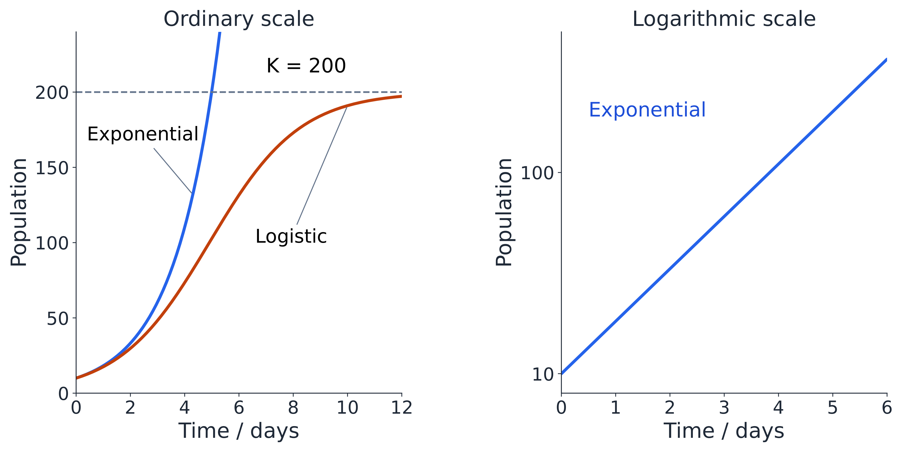
- Starting from 10 with daily doubling gives 10, 20, 40, 80 and 160 over days zero to four. The additions grow, while the proportional rate stays constant. A logarithmic population axis makes a constant exponential phase approximately straight; zero and negative counts cannot be logged.
- In a logistic model, per-capita growth falls as population approaches carrying capacity; at the capacity, gains and losses balance in the ideal model. The sigmoid curve need not begin with a flat lag phase. A short exponential-looking segment does not establish indefinite growth, and real populations may overshoot and decline.
An invented exponential model starts at 10 organisms at day zero and doubles once each day. Find the model population at day four.
Difficulty 2/5 · 140 coins + a small bonus on first completion today
10 × 2⁴ = 160. The model multiplies repeatedly, rather than adding ten each day; it is not a claim of indefinite resource-free growth.
Test a growth model without forcing every population onto it
- An approved duckweed study can count consistently defined fronds over time in independent vessels. Control starting number, medium, vessel area, light and temperature, then examine the plot and early logarithmic trend. Repeated counts of one vessel do not replace biological replication across vessels.
- Klein's St Matthew Island study reports 29 introduced reindeer in 1944, about 6,000 in 1963 and 42 counted in 1966. The crash occurred during winter 1963–64, with depleted food and extreme conditions interacting. The 1966 count is not the crash date, and 6,000 is not a demonstrated stable carrying capacity.
Compare cooperation, competition and community membership
- Members of one species can compete for limiting resources and cooperate in other tasks: red deer compete for mates, crowded pines for resources, wolves cooperate in hunting, and penguin huddles reduce heat loss. A species is not exclusively cooperative or exclusively competitive in all circumstances.
- A community comprises interacting populations of different species; an ecosystem also includes abiotic conditions and exchanges. Herbivory removes plant tissue, predation typically kills prey during feeding, parasites benefit at a living host's expense, and pathogenicity concerns disease. Categories can overlap; naming one does not measure its effect on the whole community.
Name both benefits in a mutualism
- In compatible legume root nodules, nitrogen-fixing bacteria provide usable nitrogen compounds; plants provide carbon compounds and a suitable environment. Nitrogen fixation does not turn nitrogen gas into glucose, and not every bacterium beside a root forms an effective nodule.
- In many reef-building corals, photosynthetic dinoflagellates supply organic products while receiving a habitat, carbon dioxide and inorganic nutrients. Light and environmental conditions affect the partnership; stress can disrupt it. Explain the transfer in both directions rather than writing only that two species “help each other”.
Qualify the orchid–fungus example by life stage
- Orchid seedlings can depend on fungal carbon before they photosynthesize. Adult green Goodyera repens provides evidence for reciprocal exchange: labelled-carbon and nitrogen work demonstrated plant-to-fungus carbon transfer and fungus-to-orchid nutrient transfer. The primary study tested actual material movement rather than inferring mutualism from proximity alone.
- Not every orchid photosynthesizes or gives the same carbon benefit to its fungus. Species, stage and conditions matter. State the demonstrated partners and exchanged materials, and separate a particular reciprocal example from a universal claim about all mycorrhizal associations.
Test introduced competition with a suitable control
- Native means occurring naturally in a region; endemic means restricted to a particular region. Introduced species have been moved beyond their natural range; only some establish, spread and become harmful invasives. Historical Dongtan comparisons found greater relative competitive ability in introduced Spartina alterniflora than native Scirpus mariqueter under studied conditions; do not automatically call the native species endemic.
- In an invented pot comparison, focal plants average 12 g alone and 8 g with a competitor, a 33.3% reduction. Randomize and replicate pots while controlling focal starting density, soil, water and pot size. A field removal also needs a sham-disturbance control; altered soil or light can contribute to a response. Co-occurrence alone cannot establish the mechanism.
In an invented controlled pot comparison, a focal species averages 12 g alone and 8 g with a competitor. Calculate percentage reduction relative to growing alone.
Difficulty 2/5 · 140 coins + a small bonus on first completion today
(12 − 8)/12 × 100 ≈ 33.3%. Randomization, independent pots and suitable density/disturbance controls affect the causal interpretation.
Calculate association from four exclusive categories
- An invented presence/absence survey has 25 quadrats with both species, 15 with A only, 15 with B only and 25 with neither. Each species is present in 40 of 80 quadrats, so every expected category count under independence is 40 × 40 / 80 = 20. Each quadrat belongs to exactly one category.
- The uncorrected chi-squared sum is four times 25/20, or 5.00. Degrees of freedom are one; using the supplied 5% critical value 3.84, reject independence. Both occur together more often than expected, but shared habitat preferences could explain this without mutualism. Adequate expected counts and independent sampling units remain necessary.
An invented independent-quadrat survey has four observed category counts 25, 15, 15 and 25. Each expected count is 20. Calculate the uncorrected chi-squared statistic Σ(O − E)²/E.
Difficulty 2/5 · 140 coins + a small bonus on first completion today
Each contribution is 5²/20 = 1.25; four give 5.00. With one degree of freedom and supplied 5% critical value 3.84, reject independence, without claiming this identifies a causal interaction.
Explain predator–prey regulation without assuming one cause
- More prey can support predator survival and reproduction; increased predation can then reduce prey growth, while later prey shortage can reduce predator success. Delayed responses can make predator peaks follow prey peaks. Neither perfect cycles nor one universal delay follows automatically.
- In the Yukon, Krebs and colleagues manipulated mammalian-predator access and food supply across large forest areas. Both treatments increased hare density, and their combination had a larger effect. This supports interacting influences; a hare–lynx graph alone cannot show that lynx are the only controlling cause.
Trace top-down and bottom-up changes through a food web
- Top-down control begins with consumer effects: increased predator pressure can reduce herbivores and release plants from grazing. Bottom-up control begins with resource or producer effects: more limiting nutrients can increase production and potentially support more consumers. Follow actual links rather than reversing a feeding arrow.
- Both can operate together, and context changes which matters most. Adding food directly for hares is not the same treatment as adding soil nutrients for plants; in the cited experiment those treatments did not give identical hare-density responses. Name the intervention, response and plausible indirect links before generalizing.
Distinguish chemical interference from resource depletion
- Sorghum root hairs release sorgoleone, an allelochemical that can inhibit other plants. Soil-fate research shows why persistence and microbial degradation matter. An inhibitory extract in a dish does not identify how much field suppression came from that chemical rather than shading, nutrients or other changes.
- Antibiotic release can inhibit susceptible microbial competitors. Penicillin-producing Penicillium rubens is a fungal example; penicillin interferes with bacterial wall synthesis, not a human cell wall. Taxonomic work identified Fleming's strain as P. rubens. Producer, target and mechanism differ, and laboratory inhibition does not guarantee the same exposure in every soil.
Match an ecological conclusion to its sampling and intervention
- For abundance, state boundary, sampling design, area conversion and uncertainty. For recapture, explain mixing and the effect of mark loss. For growth, separate the observed curve from its proposed causes and check whether resources, movement or interactions changed.
- For association, calculate the appropriate categories and qualify the result; a significant statistic does not identify a mechanism, and failure to reject is not proof of no interaction. For competition or food-web control, compare interventions and suitable controls, specify independent units and explain each causal link. Use low-impact approved methods or supplied simulations.
A crowded-edge survey, a significant co-occurrence test and a food-addition response are used to claim an exact population size and one universal ecological cause. Evaluate the reasoning and suggest stronger evidence.
Sampling estimates abundance; statistical association describes a pattern; controlled interventions can test specific influences. Their conclusions have different limits.
Define stability through a property and a timescale
- A forest can persist while trees die, seedlings establish and populations fluctuate. Stability concerns important properties and processes over a stated interval, rather than unchanged individuals. Resistance is limited change under disturbance; resilience is capacity to recover. Canopy cover, productivity, composition and nutrient retention need not recover together.
- Wing and colleagues' Cerrejón fossils document a Colombian rainforest flora about 58 million years old, with plant families important in modern Neotropical forests. This supports long persistence of rainforest organization, not an unchanged species list or one continuously identical local community. Match the timescale and evidence to the claim.
Connect continuing energy input with nutrient recycling and diversity
- Most ecosystems require continuing light input because transferred energy eventually dissipates as heat. Nutrients can cycle through organisms and the non-living environment; energy does not cycle in the same way. Decomposers release mineral nutrients while primary production supplies organic matter to food webs.
- Genetic and species diversity can provide different responses or partly overlapping functions after disturbance, supporting resilience without guaranteeing protection from every event. Water supply, temperature and disturbance frequency must remain within tolerable limits. Logistic growth of one population does not alone establish stability of every ecosystem property, and carrying capacity depends on conditions.
Trace reinforcing forest feedback without inventing a tipping threshold
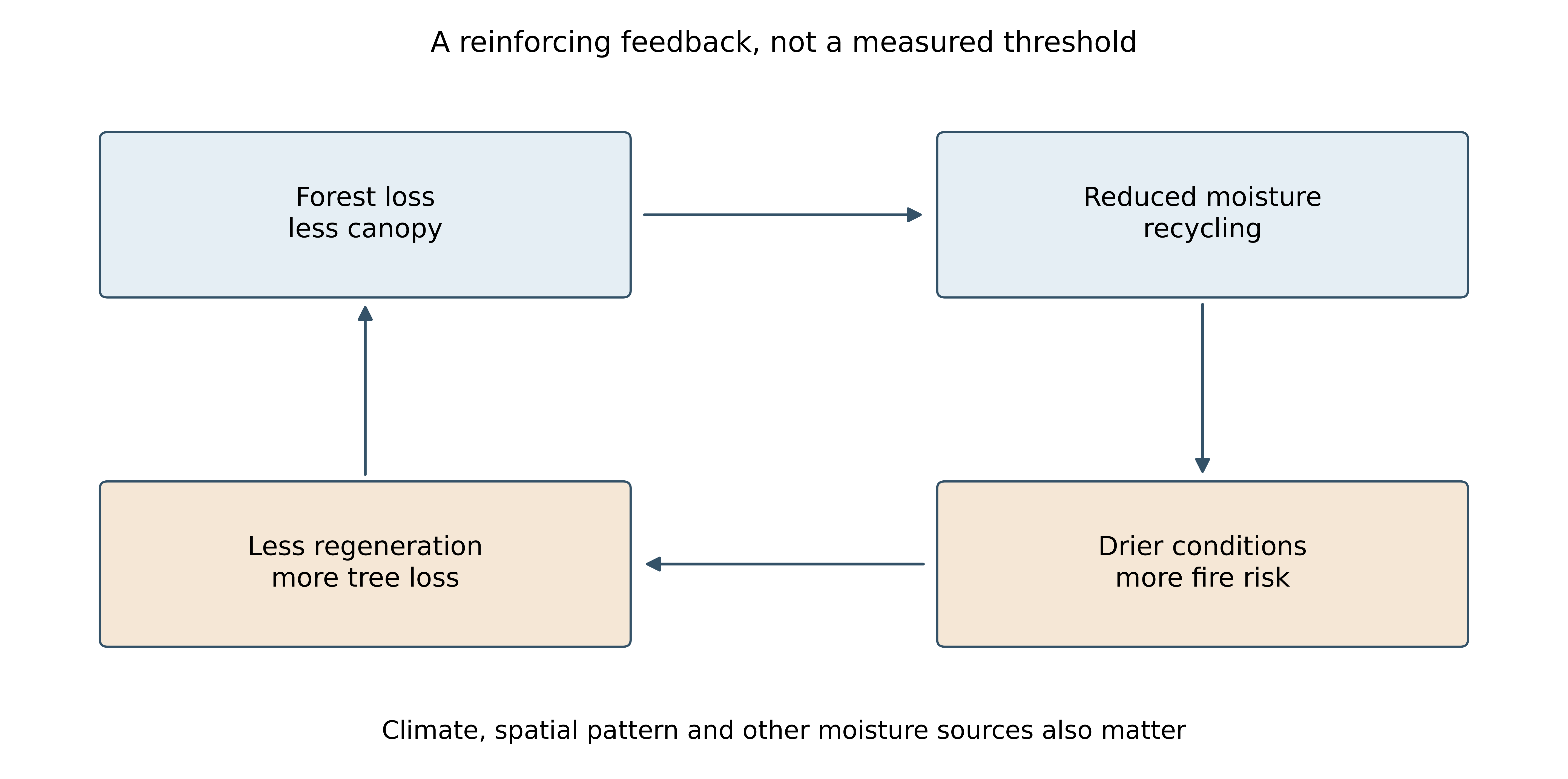
- Trees return water vapour through transpiration, while evaporation, atmospheric transport, condensation and ocean-derived moisture also contribute to rainfall. Forest removal can weaken moisture recycling and change surface heating. Drier conditions can impair regeneration and favour fire, reinforcing forest loss. These arrows represent causal effects, not food-web energy transfer.
- A tipping point is a threshold beyond which additional pressure can trigger a large persistent state change. Spatial pattern, drought, fire and climate affect the risk; the diagram supplies no single measured Amazon-wide cut-off. Flores and colleagues' analysis explicitly discusses interacting drivers and uncertainty. An invented area decline from 12,000 to 9,000 square kilometres is 25%; a further decline to 8,400 is 6.67% of 9,000, but five percentage points of the original area.
An invented forest region declines from 12,000 to 9,000 square kilometres, then to 8,400. Find the second decline as a percentage of the 9,000-square-kilometre starting area for that interval.
Difficulty 2/5 · 140 coins + a small bonus on first completion today
600/9,000 × 100 ≈ 6.67%. It is also five percentage points of the original 12,000; the baseline must be specified.
Set the matter and energy boundary of a mesocosm
- A mesocosm is a contained ecosystem model including interacting organisms and physical conditions. A sealed transparent plant–microbial vessel can be closed to matter while exchanging light and heat; it is not isolated from energy. An open tank has different inputs and losses. Define the boundary before drawing an oxygen or nutrient budget.
- A light comparison needs independent replicate vessels, random treatment allocation and matched water, starting community, nutrients, temperature and headspace. Repeated sensor readings do not create additional independent vessels. Use teacher-approved organisms and maintenance criteria; do not seal animals into a system expected to become oxygen-depleted. Supplied data can be analysed without creating that risk.
Which boundary description fits a sealed transparent plant–microbial mesocosm exposed to light and exchanging heat?
Difficulty 1/5 · 100 coins + a small bonus on first completion today
Matter closure is distinct from energy isolation. Repeated measurements do not create extra independent vessels.
Interpret mesocosm oxygen as a net balance
- In the invented light treatment, oxygen production and consumption can approximately balance. In darkness, photosynthetic oxygen production stops while respiration continues. A decline from 8.0 to 1.4 mg/L over four days is a 6.6 mg/L change, averaging a net fall of 1.65 mg/L per day.
- Stable oxygen does not mean no respiration, and a fall does not separately quantify every species' consumption. Sensor drift, unequal starting biomass and temperature differences can alter the pattern. The figure supplies means without uncertainty; a short stable record does not prove indefinite stability in a small system with simplified food webs and limited buffering.
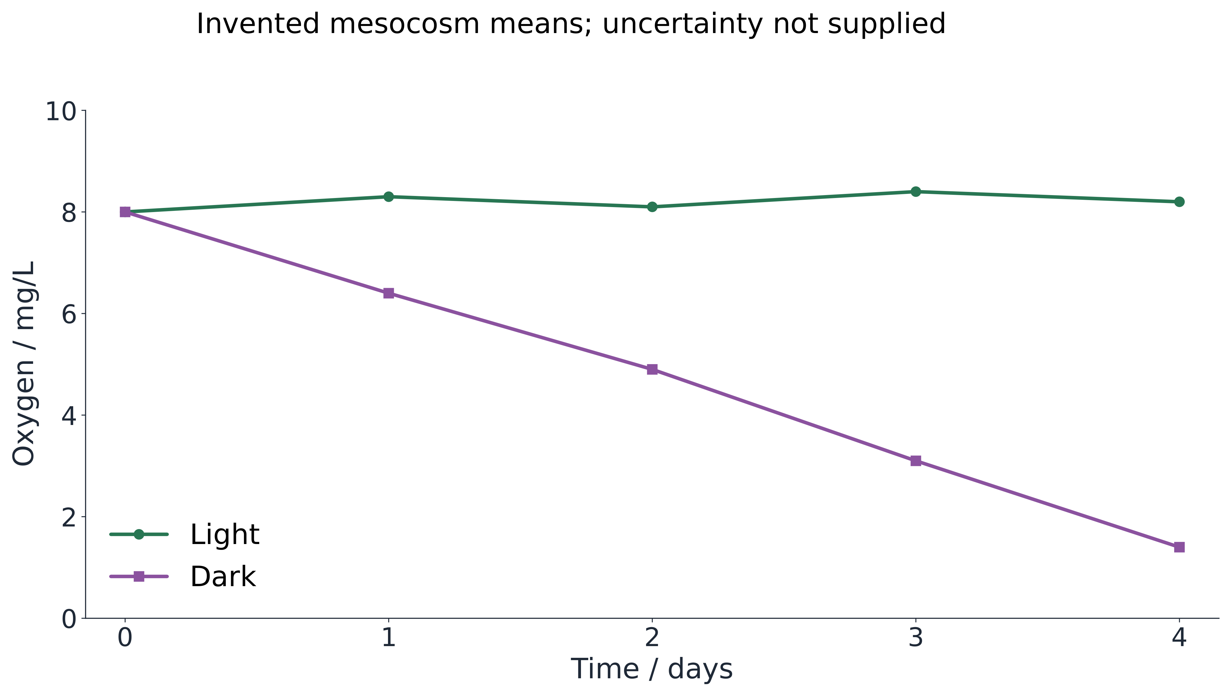
Invented dissolved oxygen falls from 8.0 to 1.4 mg/L over four days in a dark mesocosm. Find the magnitude of the average net fall per day.
Difficulty 2/5 · 140 coins + a small bonus on first completion today
(8.0 − 1.4)/4 = 1.65 mg/L per day. This is a net concentration-change rate, not separate direct measurements of every species’ respiration.
Explain a keystone effect through an indirect interaction
- A keystone species has a community effect disproportionate to its abundance; it need not be the most numerous species. In North Pacific nearshore systems, sea otters consume sea urchins, which graze kelp. Reduced grazing can support kelp and the habitat it provides. The US Fish and Wildlife Service account describes this indirect effect.
- Other predators, urchin behaviour, storms and temperature also matter, so one simple cascade is not guaranteed on every coast. Compare suitable control sites or before/after records and measure the intermediate grazing response. An otter–kelp correlation alone does not exclude a shared environmental cause or show every link in the mechanism.
Apply a harvesting balance with a conditional replacement rate
- A renewable resource can regenerate yet still be depleted. In an invented fish stock, current biomass 1,000 tonnes plus annual net replacement 100 minus harvest 150 gives 950 after one year and 900 after two if the rates remain constant. If all other gains/losses are included, the annual change is −50 tonnes.
- From 900 tonnes, replacement 120 and harvest 80 give +40 per year and 1,020 after three years under that model. Real replacement changes with stock size, age structure, food, temperature and mortality. A precautionary harvest margin addresses uncertainty; matching one estimated year's replacement does not guarantee indefinite sustainability.
An invented fish biomass starts at 1,000 tonnes, with annual net replacement 100 tonnes and harvest 150 tonnes. If these rates stay constant, what biomass remains after two years?
Difficulty 2/5 · 140 coins + a small bonus on first completion today
Annual change = 100 − 150 = −50 tonnes; 1,000 − 2 × 50 = 900. Real replacement can depend on stock size and conditions, so the model is conditional.
Measure recruitment and fishing effort rather than mature abundance alone
- Brazil nut trees can survive as adults while too few juveniles replace them. Peres and colleagues' 23-population study linked persistent intensive harvesting with poor juvenile representation. Assess seedlings, juveniles, reproductive adults and harvest history, while considering habitat and sampling differences. Harvesting seeds can affect the next generation before adult numbers visibly fall.
- For a marine stock such as Atlantic cod, assessment needs recruitment, spawning biomass, age/size structure, landings, discards, mortality and survey evidence. Catch alone depends on effort and technology as well as abundance; a protective quota can also lower catch. Do not merge every regional stock into one population or infer unchanged abundance from unchanged landings.
Include soil and exported nutrients in agricultural comparisons
- Removing crops exports nutrients that must be replenished. Mineral fertilizer, organic inputs and nitrogen-fixing associations contribute differently; their use still needs a nutrient budget. Soil erosion removes material and can impair future productivity. Crop yield in one season does not quantify all changes in soil or downstream water.
- Compare production with nutrient input/loss, soil cover and structure, water use and biodiversity effects. A monoculture can simplify food webs and share susceptibility to a pest. Use defined outcomes and timescales rather than labelling every input harmful or assuming a higher immediate yield proves sustainable production.
Trace nutrient enrichment through decomposition to oxygen stress
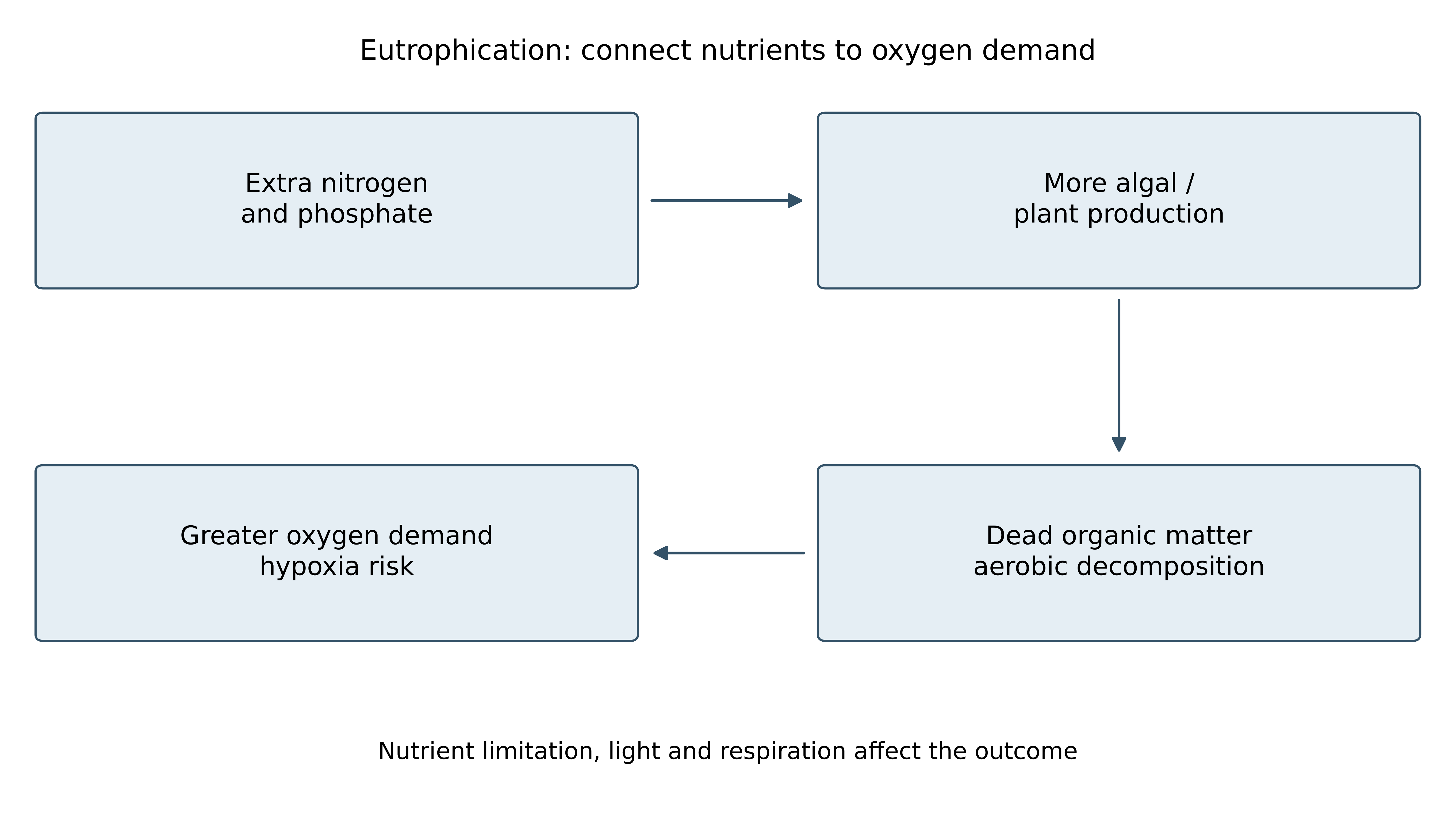
- Nitrogen or phosphate reaching water can increase production when the supplied nutrient limits growth. A bloom can shade submerged producers. Living organisms respire, and dead organic matter supports aerobic decomposers that consume dissolved oxygen. Increased organic supply can raise oxygen demand and contribute to hypoxia.
- Fertilizer does not simply poison every oxygen molecule. Daytime photosynthesis can temporarily raise oxygen; night-time respiration and decomposition after bloom decline can lower it. Buffer strips, reduced nutrient losses and wastewater treatment address inputs, but stored nutrients and altered food webs can delay recovery. Measure nutrients, oxygen and relevant conditions rather than colour alone.
Keep a five-day oxygen-demand result separate from a daily rate
- In a simplified undiluted dark test over five days at 20 degrees Celsius, oxygen falling from 8 to 3 mg/L gives biochemical oxygen demand over that interval of 5 mg/L. A matched sample falling from 8 to 6 gives 2 mg/L. These are concentration differences under defined conditions, not automatically rates of 5 and 2 mg/L per day.
- Formal methods may need dilution and seed corrections. Match starting oxygen, temperature and duration when comparing samples, and state whether those corrections apply. A larger result indicates greater consumption in the test, not a direct census of decomposers or proof that all field oxygen changes have the same cause.
In the stated simplified undiluted five-day dark test, dissolved oxygen changes from 8 to 3 mg/L. Find the oxygen demand over the test interval, with no dilution or seed correction required in this model.
Difficulty 2/5 · 140 coins + a small bonus on first completion today
8 − 3 = 5 mg/L over the specified five-day test. The result is not automatically 5 mg/L per day; formal methods may require additional corrections.
Distinguish pollutant build-up within organisms from trophic magnification
- Bioaccumulation is build-up within an organism when uptake exceeds elimination. Biomagnification is increasing concentration between trophic levels, often through repeated dietary intake and slow elimination. Invented wet-tissue concentrations 0.02, 0.10, 0.50 and 2.00 mg/kg give successive ratios 5, 5 and 4; the overall ratio is 100, not a universal tenfold rule at every step.
- DDE, a persistent DDT breakdown product, is associated with eggshell thinning in susceptible birds. Methylmercury is important in aquatic food-web accumulation; chemical forms of mercury do not behave identically. Compare equivalent tissue mass, age and exposure history. More total pollutant in a large animal is not itself a higher concentration, and trophic transfer does not create pollutant atoms.
Invented wet-tissue pollutant concentrations are 0.02 mg/kg in producers and 2.00 mg/kg in predatory fish. Find the predator-to-producer concentration ratio.
Difficulty 2/5 · 140 coins + a small bonus on first completion today
2.00/0.02 = 100. Compare equivalent tissue and exposure conditions; this ratio does not create new pollutant atoms or establish a universal increase per trophic step.
Match a plastics claim to the measured harm and exposure
- Nets, lines and packaging can entangle animals; ingested items can obstruct or injure digestive pathways and interfere with feeding. Effects depend on size, shape, organism and exposure. Microplastics are commonly defined as particles below 5 mm; small fragments and fibres can be ingested and enter food webs.
- Fragmentation makes smaller particles without necessarily mineralizing the polymer. Different polymers need not behave identically, and detection of a particle does not by itself establish a population decline. A striking image documents an event rather than its prevalence. Standardized litter surveys, organism observations and intervention comparisons support stronger claims about avoiding releases or gear loss.
Evaluate rewilding through restored processes and monitored outcomes
- Rewilding can restore interactions, reconnect habitats and reduce pressures preventing regeneration. At Hinewai Reserve in New Zealand, native regeneration proceeds with limited interference while selected damaging introduced organisms are controlled. Introduced gorse can temporarily nurse native seedlings there; this is not a general instruction to retain every introduced species everywhere.
- Choose measurable outcomes such as recruitment, connectivity, water quality or recovered interactions. Suitable comparisons and repeated monitoring help distinguish management from background change. Reintroductions need evidence about habitat and ecological roles as well as conflict, disease and invasion risks. A short visit or one attractive species does not establish whole-system recovery.
Explain how ecosystem stability can coexist with continuing change. Use a mesocosm, a harvested resource and a restoration example to distinguish a measured outcome from a stronger untested claim.
Name the property, process, boundary and timescale before claiming system persistence or management success.
AHL: Separate primary and secondary succession by their starting conditions
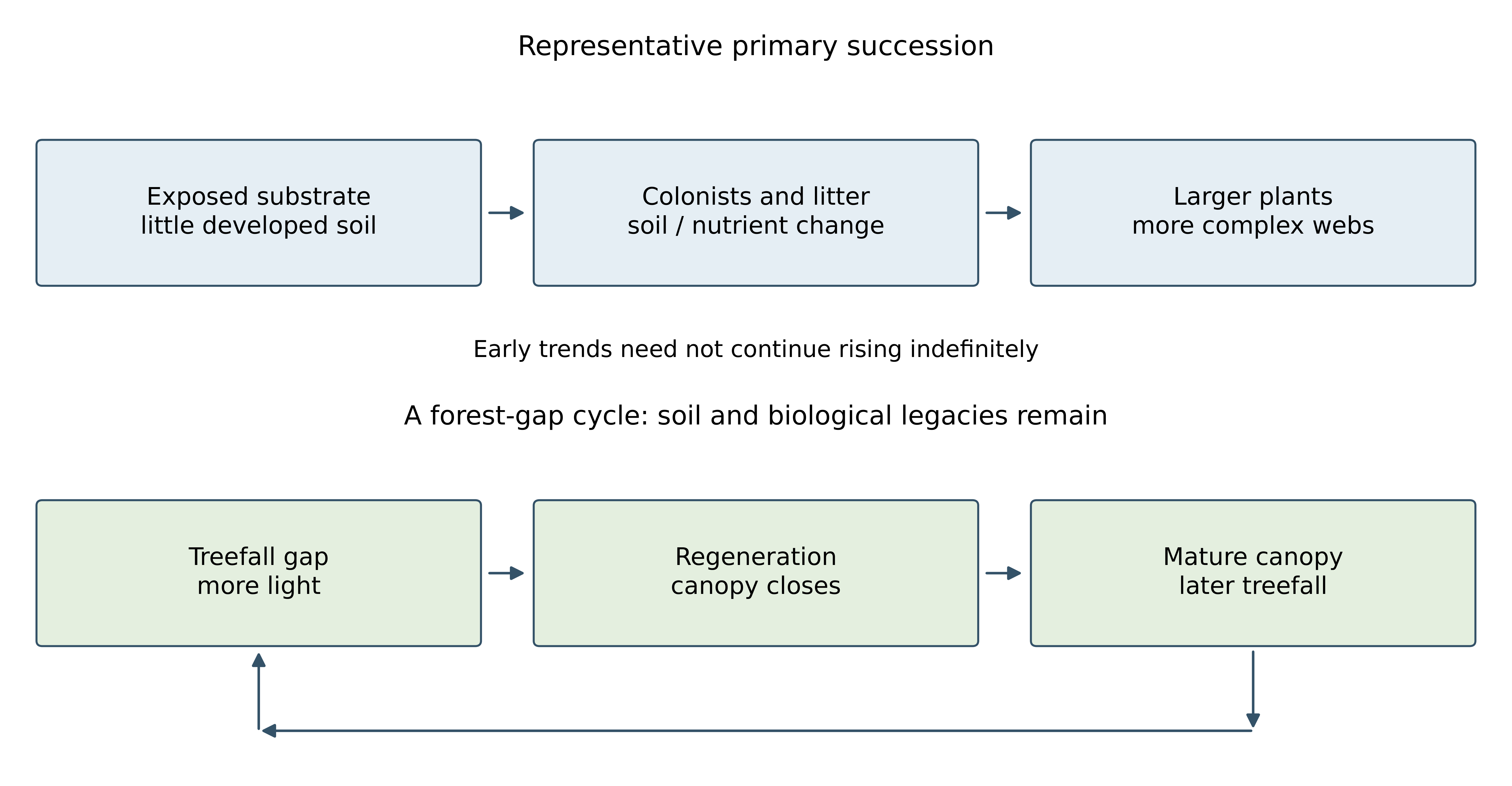
- Succession changes community composition as conditions and interactions change. New substrate, altered water levels and fire can provide abiotic triggers; colonists also alter shade, litter and nutrients. Primary succession begins with little or no developed soil, while secondary succession retains soil and biological legacies after disturbance.
- A forest canopy gap is not a new bare-rock surface simply because light increases. Starting conditions affect establishment, growth and pathways. Distinguish a community's sequence from one individual's development, and avoid treating every disturbance as a reset to identical initial conditions.
AHL: Which comparison correctly distinguishes succession after a new glacial surface is exposed from succession after a forest canopy gap?
Difficulty 1/5 · 100 coins + a small bonus on first completion today
Starting substrate, soil and biological legacies matter. Changed light alone does not erase the existing system.
AHL: Connect developing soil with multiple successional pathways
- On exposed glacial material, weathering and organic inputs help soil develop. Suitable nitrogen-fixing associations, including alder with Frankia bacteria, can increase nitrogen supply. Larger plants, litter, consumers and decomposers can support more complex production and cycling. Early increases in size, diversity or productivity need not continue forever or monotonically.
- Fastie's 1995 Glacier Bay reconstruction, using tree-ring histories, found multiple pathways associated with landscape context and seed arrival. Different-aged sites do not automatically represent consecutive stages of one universal history. A chronosequence needs comparable starting conditions and relevant controls; repeated observations strengthen the inference.
AHL: What does Fastie’s Glacier Bay reconstruction warn against when comparing sites exposed at different dates?
Difficulty 1/5 · 100 coins + a small bonus on first completion today
Multiple pathways associated with context and arrival history qualify space-for-time inference. Different-aged sites need comparability rather than automatic treatment as consecutive stages.
AHL: Explain cyclical succession as a patch mosaic
- A treefall gap in a temperate beech forest admits more light, changing ground vegetation and tree regeneration. Growth closes the canopy and restores shade; later treefall can restart a similar community cycle. The change involves interacting species and conditions, rather than only one tree growing older.
- Patches at different stages can coexist within a persistent forest, so stable broad properties can accompany local community change. There is no fixed universal cycle duration. Severe disturbance can redirect a pathway, and measuring one patch is not necessarily representative of the whole landscape.
AHL: Connect persistent communities with continuing conditions and management
- A climax community is a relatively persistent later-successional community under prevailing conditions, not an eternal species list. Climate, disturbance, dispersal and local conditions affect possible endpoints. Grazing can remove tree seedlings and maintain openness where woodland could establish, but not every natural grassland is destined to become forest.
- Drainage lowers a wetland's water table, altering oxygen, decomposition and establishment; continued drainage can arrest wetland recovery. Reducing grazing or restoring hydrology may permit change, subject to soils, seed sources, other pressures and time. Explain the mechanism keeping a community in its current state and monitor the process after intervention, rather than assuming one management action guarantees recovery.
AHL: Compare a new glacial surface, a recurring beech-forest gap and a drained wetland. Explain processes of community change, one source of divergent pathways and one measurable test of management.
The initial state and continuing drivers determine possible trajectories; one endpoint label does not replace a causal explanation.