| Enduring Understanding | Learning Objective | Essential Knowledge |
|---|---|---|
PRD-4 | PRD-4.A |
|
Factor Markets
AP Microeconomics · Topic 5
 7:56
7:56
Factor Markets
Two workers. One sews shirts in a clothing factory. The other builds cars on an assembly line. The second earns far more. Why? In this unit the firm is the…
English narration · English + 中文 subtitles burned in
5.1
Introduction to Factor Markets
Syllabus
Source: College Board AP Course and Exam Description
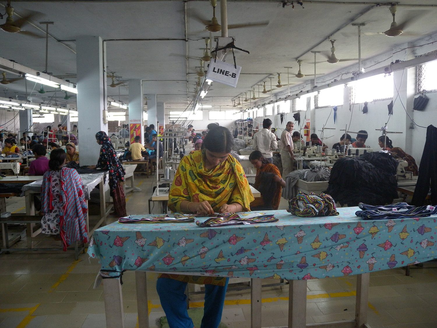
A bakery sells bread but buys flour and hires workers. The bread market concerns its output; the labour market concerns an input. In a factor market 要素市场, firms demand the services of factors of production: labour, land and capital. In the basic circular-flow model, households supply factors and receive wages, rent and other factor income. Workers are not products that the firm owns.
Demand for an input is derived demand 派生需求: firms want the revenue its output brings. If customers want more bread and its price rises, a worker's extra loaves may bring more revenue. More valuable output can increase labour demand, with productivity and other conditions unchanged.
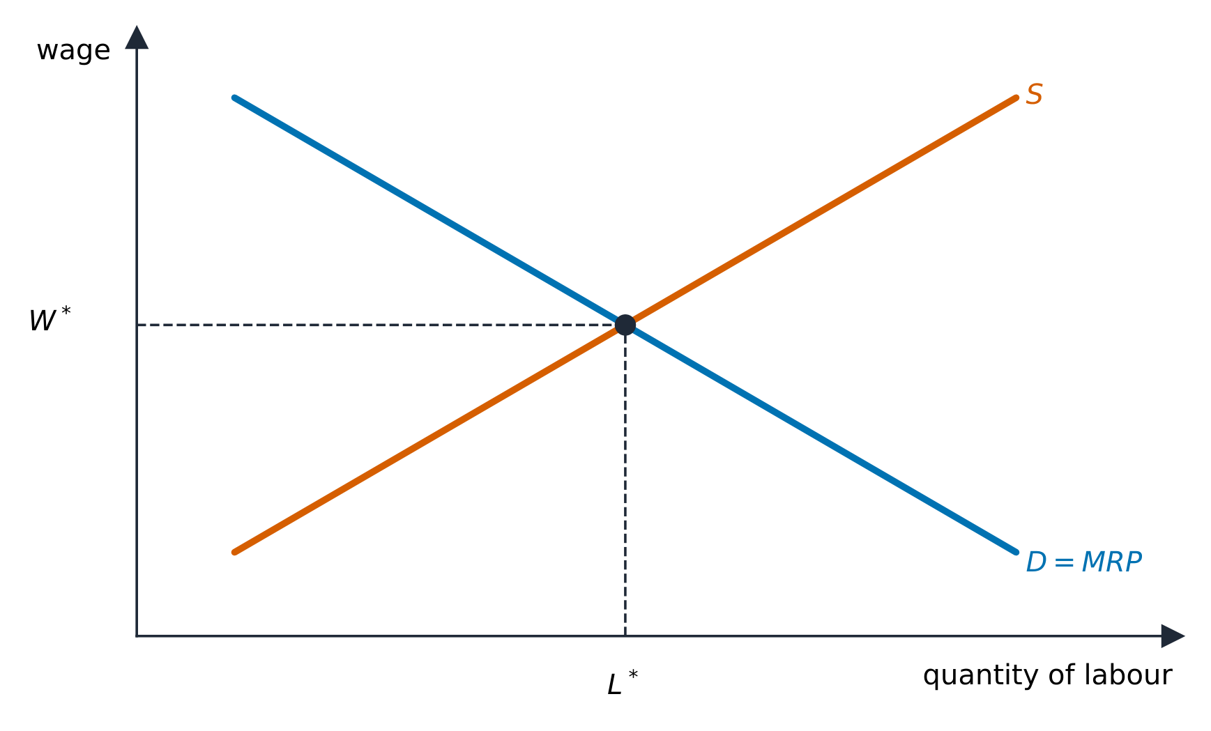
A change in the wage itself is a movement along labour demand or supply. A change in output price, worker productivity or the availability of workers shifts a curve. Keep the labour market, the firm's hiring decision and the product market distinct.
Explore
A labour (factor) market
In a factor market firms demand labour and households supply it; the wage settles where demand meets supply. Shift either curve and watch the wage and employment move.
Vocabulary
Train
| English |
|---|
| factor market/ˈfæktə ˈmɑːkɪt/ |
| derived demand/dɪˈraɪvd dɪˈmænd/ |
5.2
Changes in Factor Demand and Factor Supply
Syllabus
| Enduring Understanding | Learning Objective | Essential Knowledge |
|---|---|---|
PRD-4 | PRD-4.B |
|
Source: College Board AP Course and Exam Description
Labour demand. A higher output price in a competitive product market raises the revenue from each extra unit of output. Better training or complementary equipment can raise workers' marginal product. Both can shift labour demand right, holding other conditions constant. Technology that replaces workers can instead reduce demand for a particular job.
A cheaper substitute input, such as a robot, has two possible effects. Substitution toward robots can reduce labour use for a given output. Lower production cost can also expand output and increase demand for workers. The net effect needs evidence; do not assume every cheaper machine raises or lowers labour demand.
Labour supply. More qualified workers, training that allows entry into an occupation, or immigration can shift supply right. Better wages in other available jobs can shift supply left for this occupation. Working conditions, preferences and the availability of alternatives matter. A higher wage in this occupation alone changes quantity supplied along the existing curve.
One competitive market
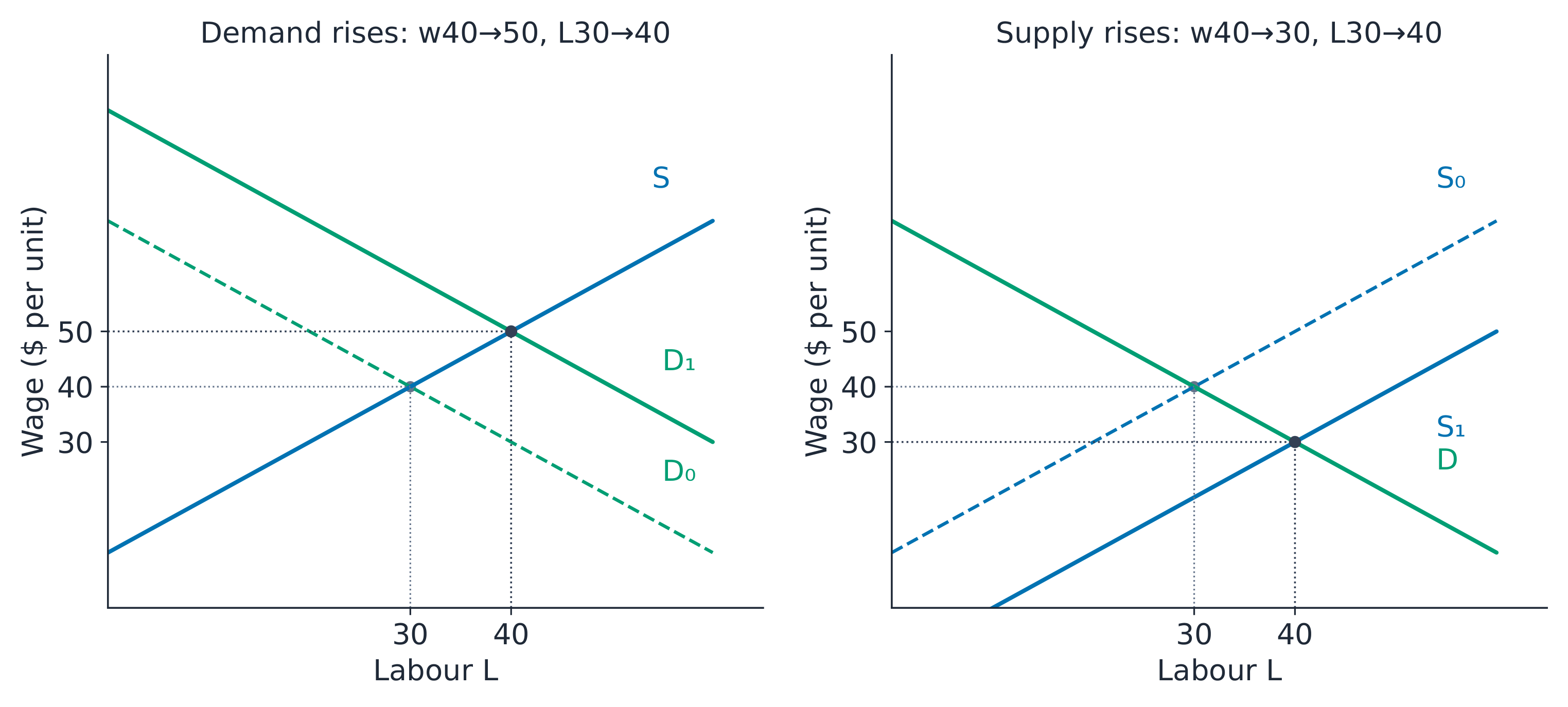
Write demand as $w=70-L$ and supply as $w=10+L$. Wage $w$ is dollars per labour unit per period; $L$ is market labour in those units. Equating demand and supply:
$$70-L=10+L\quad\Rightarrow\quad L=(70-10)/2=30$$
$$w=10+L=10+30=\$40$$
Now compare two separate changes from that baseline.
| Change | New equation | Labour L | Wage w |
|---|---|---|---|
| Higher labour demand | Demand: w=90−L | 40 | $50 |
| More available workers | Supply: w=−10+L | 40 | $30 |
For higher demand, $90-L=10+L$ gives $L=40$, then $w=50$. For higher supply, $70-L=-10+L$ gives $L=40$, then $w=30$. The new supply equation is used only in the relevant nonnegative-wage range. Both changes raise employment, but their wage effects differ.
If demand and supply both shift right, employment rises in the standard model, but the wage change depends on their relative shifts. Here, shifting demand to $90-L$ and supply to $-10+L$ gives $L=50$, $w=40$. Wage staying unchanged is one possible outcome, not a general rule.
5.3
Profit-Maximizing Behavior in Perfectly Competitive Factor Markets
Syllabus
| Enduring Understanding | Learning Objective | Essential Knowledge |
|---|---|---|
PRD-4 | PRD-4.C |
|
Source: College Board AP Course and Exam Description
A firm compares extra revenue with extra labour cost. Marginal revenue product 边际收益产品 is extra revenue per extra labour unit: $MRP=\Delta TR/\Delta L$.
At the margin, $MRP=MP_L\times MR$. Only in a perfectly competitive product market does $MR=P$, allowing $MRP=MP_L\times P$. Being a wage taker 工资接受者 in the labour market does not prove the firm is a price taker for its output.
For example, if marginal product is 5 units and marginal revenue is $\$6$ per unit, MRP is $5\times\$6=\$30$ per labour unit. An output price of $\$10$ would give value of marginal product $\$50$, but would not make MRP $\$50$ when MR is $\$6$. At a marginal labour cost of $\$40$, this extra labour is not profitable.
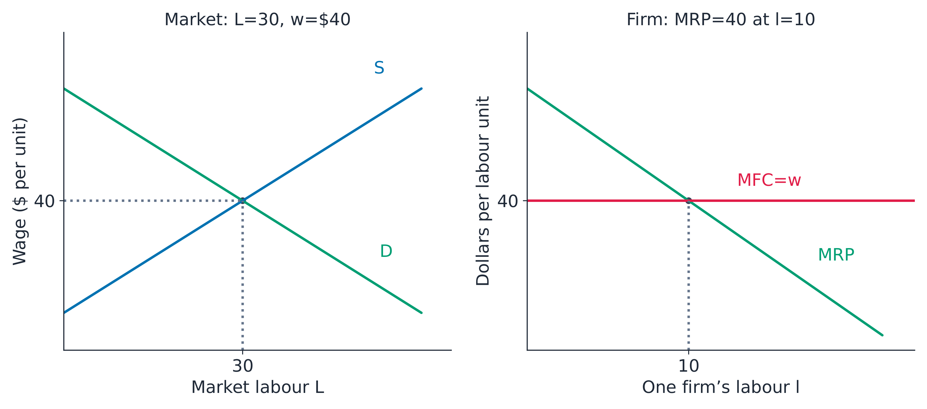
Marginal factor cost 边际要素成本 (MFC) is the extra total input cost divided by the extra input hired. In a perfectly competitive labour market, a small firm can hire at the market wage without raising it, so its MFC equals that wage and is horizontal. In a smooth model with falling MRP and a suitable crossing, the firm chooses $MRP=MFC$. With whole workers, compare the last worker included and the next excluded; exact equality is not required.
The market above sets $w=\$40$. One firm's MRP is $70-3l$. Its hiring decision is:
$$MRP=w\quad\Rightarrow\quad70-3l=40$$
$$l=(70-40)/3=10\text{ labour units}$$
Three identical firms of this type would together demand $L=30$ at that wage. Do not draw the upward-sloping market supply curve as a small wage-taking firm's supply curve.
Hiring whole workers from a production table
Use a separate bakery case. Bread sells in a competitive product market for $\$5$ per loaf. Workers have equal daily hours and each costs $\$25$ per day. Labour is the only variable input; daily fixed cost is $\$30$.
| Workers L | 0 | 1 | 2 | 3 | 4 | 5 |
|---|---|---|---|---|---|---|
| Loaves per day Q | 0 | 8 | 18 | 24 | 28 | 30 |
| MP: extra loaves | — | 8 | 10 | 6 | 4 | 2 |
| MRP: extra revenue | — | $40 | $50 | $30 | $20 | $10 |
Try first. Calculate worker 2's MRP. Identify where diminishing marginal returns begin. Choose workers at wage $\$25$, and calculate profit. Then consider a higher fixed cost of $\$80$.
$$MP_2=\Delta Q/\Delta L=(18-8)/(2-1)=10\text{ loaves per worker-day}$$
$$MRP_2=MP_2\times P=10\times\$5=\$50\text{ per worker-day}$$
Diminishing marginal returns begin with worker 3: MP falls from 10 to 6. MRP first rises from 40 to 50, then falls. Do not claim MRP must fall from the first worker in every table.
Hire 3 workers: the third adds $\$30$ revenue at $\$25$ cost, raising profit by $\$5$. The fourth adds only $\$20$ revenue at $\$25$ cost, reducing profit by $\$5$. No worker has MRP exactly equal to the wage; 3 is still optimal.
$$TR=P Q=\$5\times24=\$120\text{ per day}$$
$$TVC=wL=\$25\times3=\$75\text{ per day}$$
$$\pi=TR-TVC-TFC=120-75-30=\$15\text{ per day}$$
If fixed cost rises to $\$80$, hiring remains 3 because MRP and MFC do not change. Profit becomes $120-75-80=-\$35$. Operating contributes $\$45$ toward unavoidable fixed cost; not operating would lose $\$80$ this day. A lower profit alone does not change the short-run marginal hiring comparison.
Equality case. At wage $\$30$, hiring either 2 or 3 gives the same profit: $5(18)-30(2)-30=0$ and $5(24)-30(3)-30=0$. The third worker adds no net profit. Equality can mean indifference, rather than a uniquely required worker count.

The least-cost input combination
A least-cost combination 最低成本组合 produces a chosen output at the lowest possible cost. Compare marginal product per dollar spent on each input. With divisible inputs, an interior least-cost combination equates $MP_L/w$ and $MP_K/r$, where $r$ is the rental cost per capital unit. Constraints can prevent exact equality.
Suppose $MP_L=40$, $w=\$20$, $MP_K=30$ and $r=\$10$:
$$MP_L/w=40/20=2\text{ output units per dollar}$$
$$MP_K/r=30/10=3\text{ output units per dollar}$$
Capital gives more extra output per dollar at this combination. Shift spending toward capital and away from labour. For a small $\$10$ transfer, assuming these marginal products remain constant over that change, removing half a labour unit loses 20 output units; adding one capital unit gains 30. Net output rises by 10 at the same cost. Alternatively, less spending can maintain the original output. Recalculate as marginal products change.
This is cost minimization for a chosen output. It does not by itself prove the chosen output maximizes profit; that also needs revenue information.
Vocabulary
Train
| English |
|---|
| marginal revenue product/ˈmɑːdʒɪnl ˈrevənjuː ˈprɒdʌkt/ |
| marginal factor cost/ˈmɑːdʒɪnl ˈfæktə kɒst/ |
| wage taker/weɪdʒ ˈteɪkə/ |
| least-cost combination/liːst kɒst ˌkɒmbɪˈneɪʃn/ |
5.4
Monopsonistic Markets
Syllabus
| Enduring Understanding | Learning Objective | Essential Knowledge |
|---|---|---|
PRD-4 | PRD-4.D |
|
Source: College Board AP Course and Exam Description
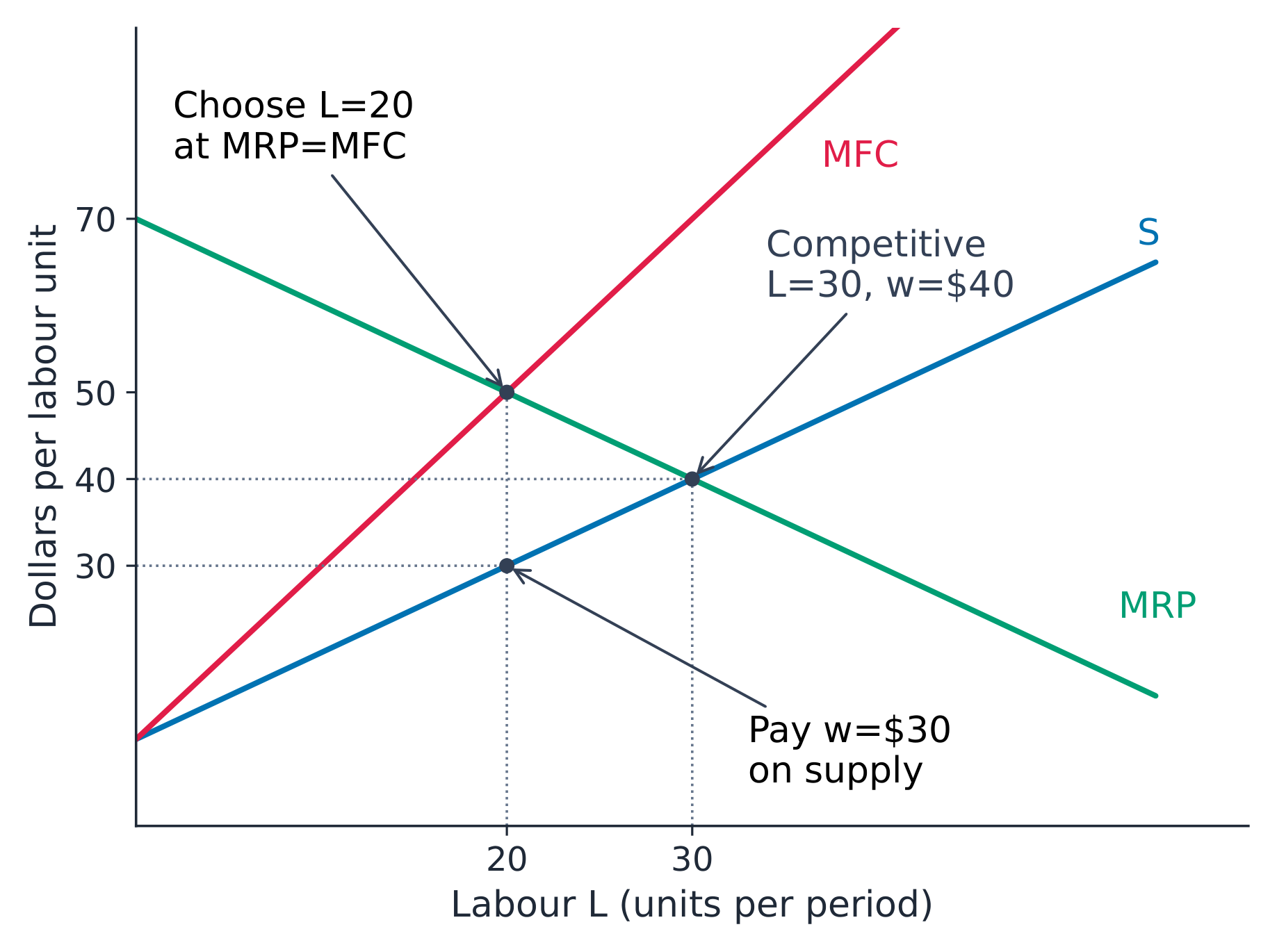
A monopsony 买方垄断 has one buyer in the relevant factor market. Consider a uniform-wage employer with supply $w=10+L$. Attracting more labour requires raising the wage for all equally paid labour units, not just the new unit.
The wage bill is $wL=(10+L)L$. In the continuous model, $MFC=10+2L$, above supply for positive employment.
Discrete wage-bill illustration. At $L=2$, wage is $\$12$ and the bill is $\$24$. At $L=3$, wage is $\$13$ and the bill is $\$39$.
$$\Delta\text{wage bill}=13(3)-12(2)=\$15$$
That extra unit costs $\$13$ for the new hire plus a $\$1$ raise for each of two existing units. This finite-interval cost is not the continuous MFC evaluated at the interval's endpoint.
Let MRP be $70-L$. Choose labour using the rising MFC and falling MRP:
$$MRP=MFC\quad\Rightarrow\quad70-L=10+2L$$
$$L_M=(70-10)/3=20\text{ labour units}$$
$$w_M=10+L_M=10+20=\$30\text{ per labour unit}$$
$$\text{Wage bill}=w_M L_M=30\times20=\$600\text{ per period}$$
MFC at this output is $10+2(20)=\$50$, not the wage $\$30$. Pay the wage read from supply, not from the MFC–MRP intersection.
Using the same supply and MRP as the competitive benchmark, $70-L=10+L$ gives $L_C=30$, $w_C=\$40$. The uniform-wage monopsony therefore hires fewer units at a lower wage. This comparison holds the underlying curves constant; it is not a comparison of unrelated towns or occupations.
Higher product demand. Suppose stronger demand raises output price or marginal revenue and shifts MRP to $85-L$, with labour supply unchanged. Then $85-L=10+2L$ gives $L=25$, wage $\$35$ and MFC $\$60$. The firm moves up the unchanged MFC curve; MFC of its last hired unit rises from $\$50$ to $\$60$. This is not a labour-supply shift.
Minimum wages: the level matters
A minimum wage 最低工资 is a legal floor on the wage. Return to the original monopsony MRP $70-L$ and supply $10+L$. Assume an enforced uniform wage floor, no other hiring costs and the same worker productivity.
| Wage floor | Labour hired | Wage paid | Wage bill |
|---|---|---|---|
| None | 20 | $30 | $600 |
| $35 | 25 | $35 | $875 |
| $40 | 30 | $40 | $1,200 |
| $55 | 15 | $55 | $825 |
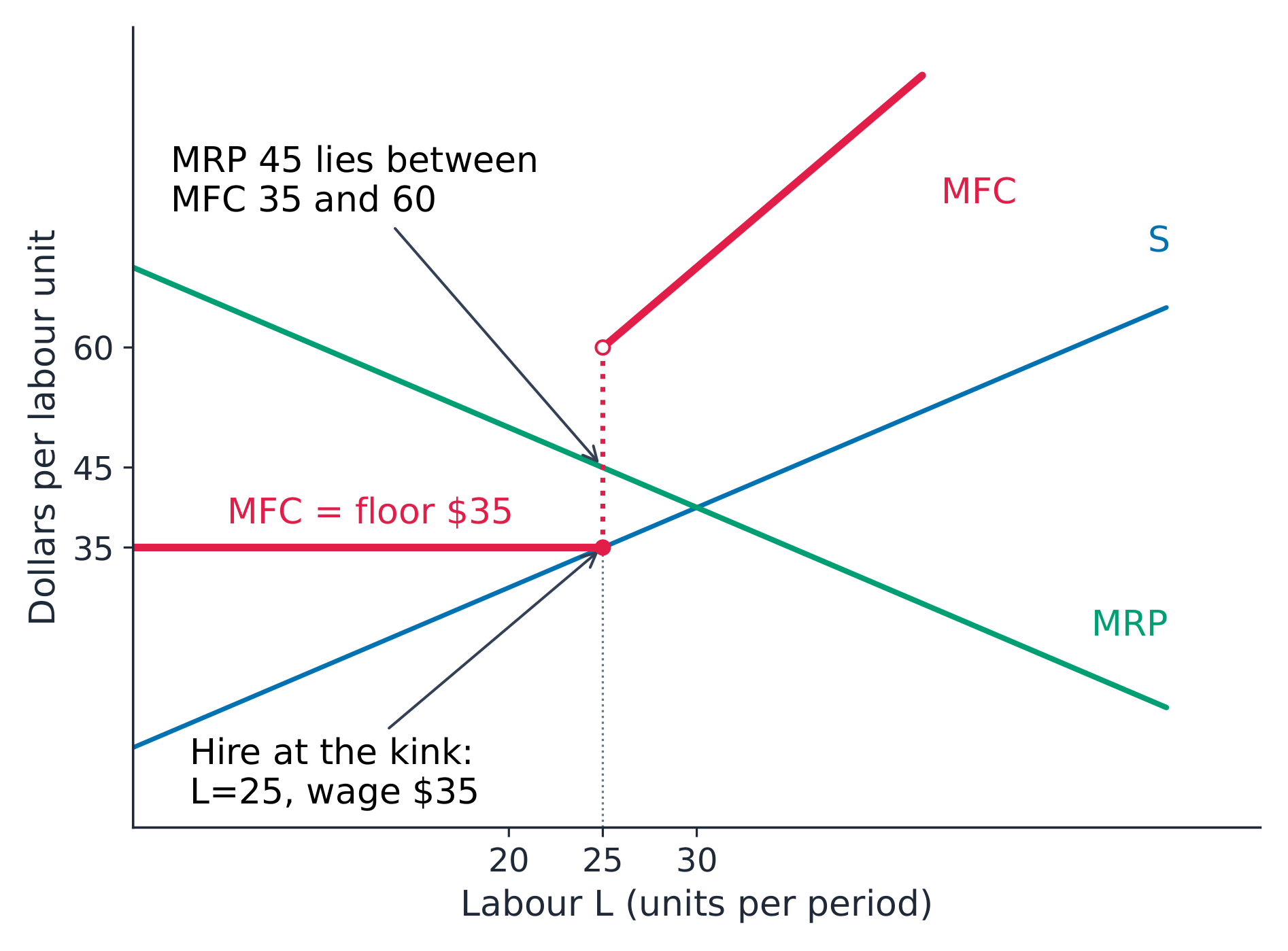
A floor of $\$35$. Supply at that wage is $L_S=35-10=25$. Up to 25 units, the employer can add labour at marginal cost $\$35$ without raising the wage of existing workers. Beyond 25, attracting additional labour requires a wage above the floor for everyone, so MFC jumps to the original $10+2L$ branch. At 25, MRP is $\$45$, between MFC just below the kink ($\$35$) and just above it ($\$60$). Profit rises up to 25 units and falls beyond it: hire 25, paying $35(25)=\$875$. There is no smooth MRP=MFC equality at the optimum kink.
A floor of $\$40$. Supply is 30; MRP there also equals $\$40$. Hiring reaches the competitive benchmark, 30 units, and the wage bill is $40(30)=\$1,200$.
A high floor of $\$55$. Labour available is 45, but demand at a marginal cost of $\$55$ is only 15: $70-L=55$ gives $L=15$. The bill is $55(15)=\$825$. Employment falls below the unregulated monopsony level of 20. A wage floor does not always raise monopsony employment.
In a competitive market with the same underlying curves, a floor above equilibrium $\$40$ creates excess labour supply. At $\$55$, supply is 45 and demand 15, a gap of 30 labour units. The monopsony result and the competitive result follow from different starting rules; do not apply a universal slogan about minimum wages.
Vocabulary
Train
| English |
|---|
| monopsony/ˈmɒnəʊpsəni/ |
| minimum wage/ˈmɪnɪməm weɪdʒ/ |
5.4
Exam tips
- State which market is competitive. Use MRP=MP×MR generally; use product price only when MR=P.
- For a worker table, calculate changes in output, value them, and compare the last included and next excluded worker with MFC. Exact equality may not exist.
- Distinguish market labour supply from a wage-taking firm's horizontal labour supply. In monopsony, choose labour at MRP=MFC but read the wage on supply.
- Rebuild the relevant MFC schedule under a wage floor. Check availability and kinks before solving an equality, then calculate wage bill as wage times labour actually hired.
Interactive lessons on this topic
Work through it step by step, with instant-check exercises.