| Enduring Understanding | Learning Objective | Essential Knowledge |
|---|---|---|
POL-2 | POL-2.A |
|
POL-2.B |
| |
POL-2.C |
|
Market Failure and the Role of Government
AP Microeconomics · Topic 6
 8:21
8:21
Market Failure and the Role of Government
Look at this factory. Somebody bought what it makes, and somebody was paid to make it. Both sides are happy with the price. But the smoke is not in that price.…
English narration · English + 中文 subtitles burned in
6.1
Socially Efficient and Inefficient Market Outcomes
Syllabus
Source: College Board AP Course and Exam Description
A factory can make a profit while its smoke harms nearby residents. The buyers and sellers may choose well for themselves but leave out a cost paid by someone else. To judge the outcome, ask whose benefits and costs the decision includes.
An allocation is socially efficient 社会有效率 when it maximizes total economic surplus, including external benefits and costs. In the standard smooth model, choose the quantity where marginal social benefit (MSB) equals marginal social cost (MSC). Below that quantity, another unit adds more benefit than cost; above it, another unit costs more than its benefit.
Market failure 市场失灵 occurs when private incentives lead to an inefficient allocation. Competition alone does not guarantee efficiency: the private and social values must also coincide. With external effects, consumer surplus plus producer surplus alone is not total social surplus. Include the external effects and, when evaluating a tax or subsidy, government revenue or spending. Transfers are not automatically resource losses.
Efficiency concerns the size of total net benefits. It does not say that the resulting distribution is fair. A change in tastes or real resource costs can change the efficient quantity; a different quantity from yesterday is not automatically a market failure.
| English |
|---|
| socially efficient/ˈsəʊʃəli ɪˈfɪʃənt/ |
| market failure/ˈmɑːkɪt ˈfeɪlɪə/ |
6.2
Externalities

Syllabus
| Enduring Understanding | Learning Objective | Essential Knowledge |
|---|---|---|
POL-3 | POL-3.A |
|
POL-3.B |
|
Source: College Board AP Course and Exam Description
An externality 外部性 is an uncompensated cost or benefit affecting a third party outside the market transaction. Private decision-makers may leave it out. A higher price paid by another buyer is not, by itself, the external cost illustrated by pollution.
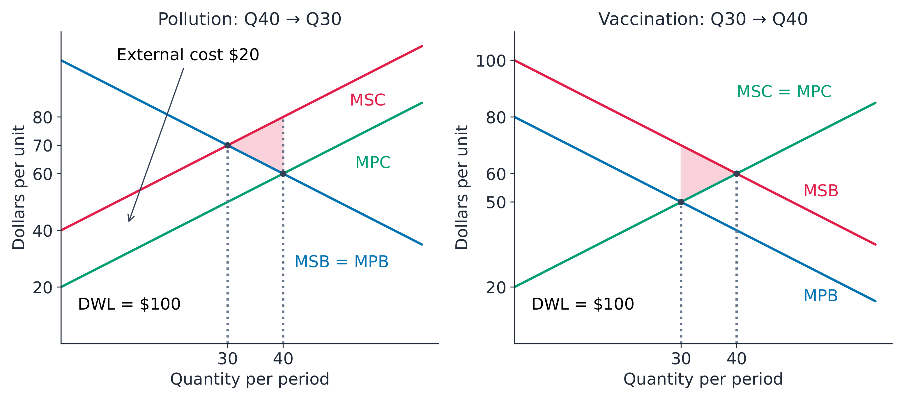
A negative externality 负外部性 can arise in production or consumption. For polluting production, MSC = MPC + marginal external cost. With no external consumption effect, MSB = MPB. A positive externality 正外部性 from vaccination can instead make MSB greater than MPB while MSC = MPC. Identify the affected side before drawing the social curve; not every externality belongs on the cost side.
Pollution: private output versus efficient output
Consider a competitive chemical market. All quantities are units per period and all marginal values are dollars per unit. Demand is MPB = MSB = 100 − Q; supply is MPC = 20 + Q. Each unit causes an external cost of $20, so MSC = 40 + Q.
Private choice. Buyers and sellers equate their private values:
Social choice. Include the pollution cost:
At Q = 30 both social marginal values are $70. The market produces ten units too many. At Q = 40, MSC is $80 but MSB is only $60. The loss is the area between social cost and social benefit over the extra units, not the entire pollution bill:
A corrective tax changes incentives
A Pigovian tax 庇古税 equal to marginal external cost at the efficient quantity can make the private choice match the social choice, under the stated model assumptions. Here a $20 per-unit tax 从量税 raises the effective supply price from 20 + Q to 40 + Q:
Buyers pay $70 and sellers keep $50; the legal payer need not bear the whole burden. Pollution still occurs: external harm is 20(30) = $600 per period. The tax does not remove every harmful unit. It removes units whose social cost exceeds social benefit.
Before tax, CS = $800 and PS = $800, but harm is $800: social net benefit is $800. After tax, CS = $450, PS = $450 and revenue is $600, while harm is $600: social net benefit is $900. The gain is the $100 deadweight loss removed. Counting the tax payment as both a cost and government revenue would count the same transfer twice.
A tax on output and a charge on emissions are different tools. If a firm can clean each unit, an emissions charge also rewards cleaner production. When harm changes with output, use marginal harm at the efficient quantity rather than an arbitrary average cost. Missing information, other market failures and enforcement costs can affect policy performance.
Vaccination: a subsidy versus a price ceiling
Now use a separate competitive market with MPB = 80 − Q, MPC = MSC = 20 + Q and a marginal external benefit of $20. Then MSB = 100 − Q. The private equilibrium is Q = 30 and P = $50; the efficient quantity is Q = 40, where MSB = MSC = $60. Lost external benefits cause underproduction.
A consumer subsidy of $20 makes the producer receive $20 more than the buyer pays:
The subsidy expands quantity to the efficient level in this model; its fiscal cost is not the same as deadweight loss. Increased product demand can also raise firms' demand for labour through MRP, as in Unit 5.
Try a different policy. A legal price ceiling of $40 gives private quantity demanded 40 but quantity supplied only 20. Without government supply or another arrangement, only 20 units can be exchanged. A lower legal price does not automatically deliver the efficient 40 units. The ceiling and the subsidy have different effects on sellers' incentives.
Other ways to address external effects
Regulation can restrict emissions or require equipment; tradable permits cap emissions and allow trading. A well-designed trading system can move abatement toward firms that can clean at lower marginal cost, but the cap, monitoring and market conditions matter. Public provision can also increase access to a service with external benefits.
The Coase theorem 科斯定理 describes how bargaining can reach an efficient allocation when rights are clear and transaction costs do not prevent agreement. The allocation of rights affects who pays whom; it need not determine the efficient activity level under these assumptions. Many affected residents, costly information or difficulty enforcing an agreement can prevent this result.

Private market response to a per-unit tax
Compare the private market quantity and prices when a per-unit tax raises supply cost. This display does not show external costs, social curves or deadweight loss; use the handout diagrams for those comparisons.
| English |
|---|
| externality/ekˈstɜːnælɪti/ |
| negative externality/ˈneɡətɪv ekˈstɜːnælɪti/ |
| Pigovian tax/pɪˈɡəʊvɪən tæks/ |
| positive externality/ˈpɒzɪtɪv ekˈstɜːnælɪti/ |
| Coase theorem/kəʊs ˈθɪərəm/ |
| per-unit tax/pɜː ˈjuːnɪt tæks/ |
6.3
Public and Private Goods
Syllabus
| Enduring Understanding | Learning Objective | Essential Knowledge |
|---|---|---|
POL-3 | POL-3.C |
|
Source: College Board AP Course and Exam Description
Rivalry 竞争性 asks whether one person's use reduces what is available to others. Excludability 排他性 asks whether non-payers can be kept out. Classify the service at the relevant capacity and under its actual access rules.
| Example | Rival? | Excludable? | Category |
|---|---|---|---|
| A sandwich | Yes | Yes | Private |
| A noncongested paid stream | No | Yes | Club |
| Open-access ocean fish | Yes | No | Common resource |
| A nonexcludable warning signal | No | No | Public |
A private good 私人物品 is rival and excludable. A public good 公共物品 is non-rival and non-excludable. People can free-ride 搭便车 when they enjoy a benefit without paying for it, weakening incentives for voluntary financing. Some public goods can still be supported by donations or other arrangements; “everyone refuses to pay” is not a definition.
One warning project. A neighbourhood signal costs $50. Three households value that single project at $30, $20 and $10. The total benefit is $60, greater than its cost, but each household values it less than paying the full $50 alone. Collective finance could support a worthwhile project that individual purchasing might not provide. This is an incentive problem, not evidence that the signal has no value.
Common resources 公共资源 are rival and non-excludable. Each fisher gains from an extra catch but can leave less stock for others. The tragedy of the commons 公地悲剧 describes inefficient overuse under such open-access incentives. Access rights, quotas or community rules may change those incentives. “Common” does not mean that every shared resource is inevitably destroyed.
Government can supply a private good free at the point of use. A school place still uses scarce classroom capacity and access can be controlled. Public funding is not the same as the economic definition of a public good.
| English |
|---|
| rivalry/ˈraɪvəlri/ |
| excludability/eksˌkluːdəˈbɪlɪti/ |
| private good/ˈpraɪvət ɡʊd/ |
| public good/ˈpʌblɪk ɡʊd/ |
| free-ride/friː raɪd/ |
| Common resources/ˈkɒmən rɪˈzɔːsɪz/ |
| tragedy of the commons/ˈtrædʒədi ɒvðə ˈkɒmənz/ |
6.4
The Effects of Government Intervention in Different Market Structures
Syllabus
| Enduring Understanding | Learning Objective | Essential Knowledge |
|---|---|---|
POL-4 | POL-4.A |
|
Source: College Board AP Course and Exam Description
Start with the market failure and the changed incentive. The same instrument can improve or worsen allocation depending on the initial conditions.
The same tax can have different welfare effects
Return to demand 100 − Q and private supply 20 + Q. With pollution cost 20, a tax 20 corrects overproduction and removes DWL100. With no external effects instead, the original Q40 is already efficient. The same tax 20 reduces output to Q30 and creates DWL100. A tax does not always create an additional efficiency loss; identify the starting social curves.
A lump-sum tax 定额税 is a fixed charge, so it does not change marginal cost or marginal revenue. For a firm that continues operating at an interior optimum, its short-run profit-maximizing quantity and price stay the same while profit falls. A lump-sum subsidy 定额补贴 raises profit without directly changing marginal incentives. Participation, entry and exit can change; the statement is not a promise of unchanged industry output forever. Changes in demand or MR can also change output even when MC stays fixed.
Regulating a natural monopoly
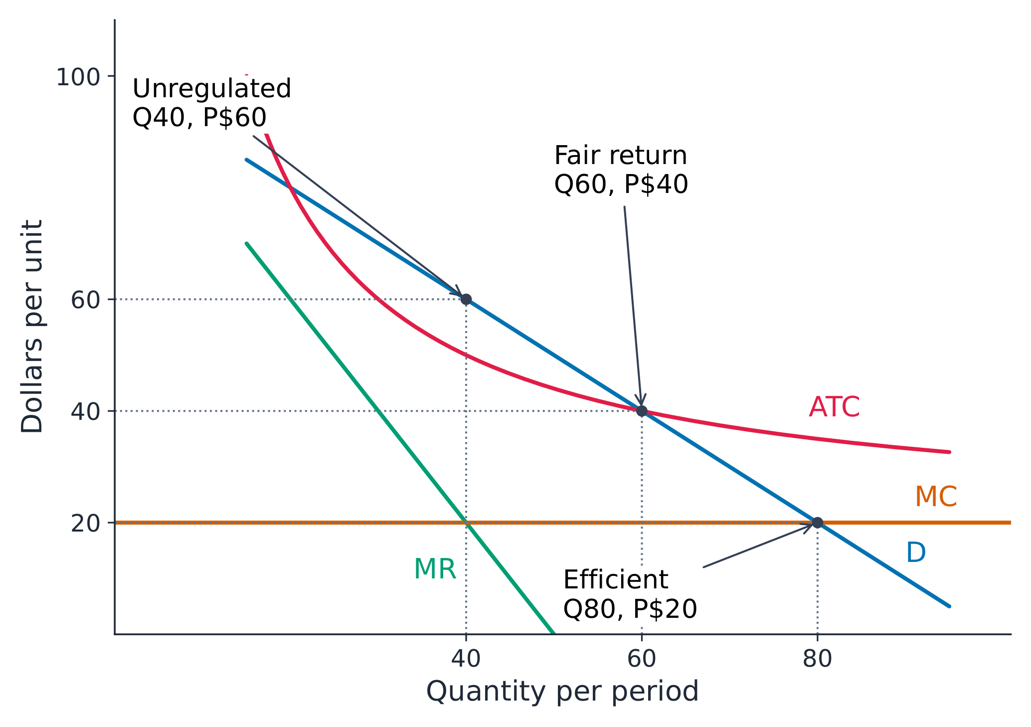
Use the separate network example from Unit 4: demand P = 100 − Q, MR = 100 − 2Q, total cost TC = 1200 + 20Q, and MC = $20. ATC = 1200/Q + 20 declines over the relevant demand range, making one producer potentially cheaper than dividing output among firms.
| Policy | Quantity | Price | Economic profit |
|---|---|---|---|
| Unregulated | 40 | $60 | $400 |
| Fair-return price | 60 | $40 | $0 |
| Marginal-cost price | 80 | $20 | −$1,200 |
The unregulated firm sets MR = MC, then reads price from demand. Fair-return pricing sets P = ATC and allows zero economic profit, but Q60 is below the efficient Q80. Its DWL is $200, compared with $800 under unregulated monopoly. Zero profit does not mean full efficiency.
Check whether a ceiling binds. Demand and ATC also meet at Q20/P80 in this model, but a ceiling of $80 is above the unregulated price $60. It leaves the firm at Q40/P60. Fair-return regulation here uses the binding ceiling $40: the firm can sell up to 60 units at that price, and each extra unit costs only $20, so it expands to Q60. This choice covers total cost. An arbitrary intersection of demand and ATC is not enough to establish the regulated choice.
Compare marginal and fixed policies. At unregulated Q40 the firm earns $400. A fixed tax 400 reduces profit to zero while leaving the interior operating choice Q40/P60 unchanged. A per-unit tax 10 instead raises effective MC to 30:
A per-unit subsidy 10 lowers effective MC to 10 and gives Q45/P55. Its profit includes the subsidy; it is $825, not just sales revenue minus original cost. Output rises, but is still below efficient Q80. A subsidy to a monopolist is not the same model as the earlier subsidy in a competitive vaccination market.
At marginal-cost pricing, revenue is $1600 and cost is $2800, so a fixed subsidy of $1200 covers the loss. Funding and administrative costs still need evaluation. A ceiling changes the firm's feasible revenue schedule; do not keep using the unregulated MR curve as if nothing had changed.
Antitrust laws 反垄断法 aim to limit anticompetitive mergers and collusion and make markets more competitive. More firms do not automatically guarantee a net gain when economies of scale are large. Evaluate the changed incentives and real costs rather than assuming every intervention succeeds.
| English |
|---|
| Antitrust laws/ˌæntɪˈtrʌst lɔːz/ |
| lump-sum tax/lʌmp sʌm tæks/ |
| lump-sum subsidy/lʌmp sʌm ˈsʌbsɪdi/ |
6.5
Inequality
Syllabus
| Enduring Understanding | Learning Objective | Essential Knowledge |
|---|---|---|
POL-5 | POL-5.A |
|
POL-5.B |
|
Source: College Board AP Course and Exam Description
Income distribution 收入分配 describes how an income flow is shared over a stated period. Wealth is a stock of assets minus liabilities at a date. High current income does not necessarily imply high accumulated wealth. Inequality compares shares; poverty concerns a living-standard threshold, so one is not a complete measure of the other.
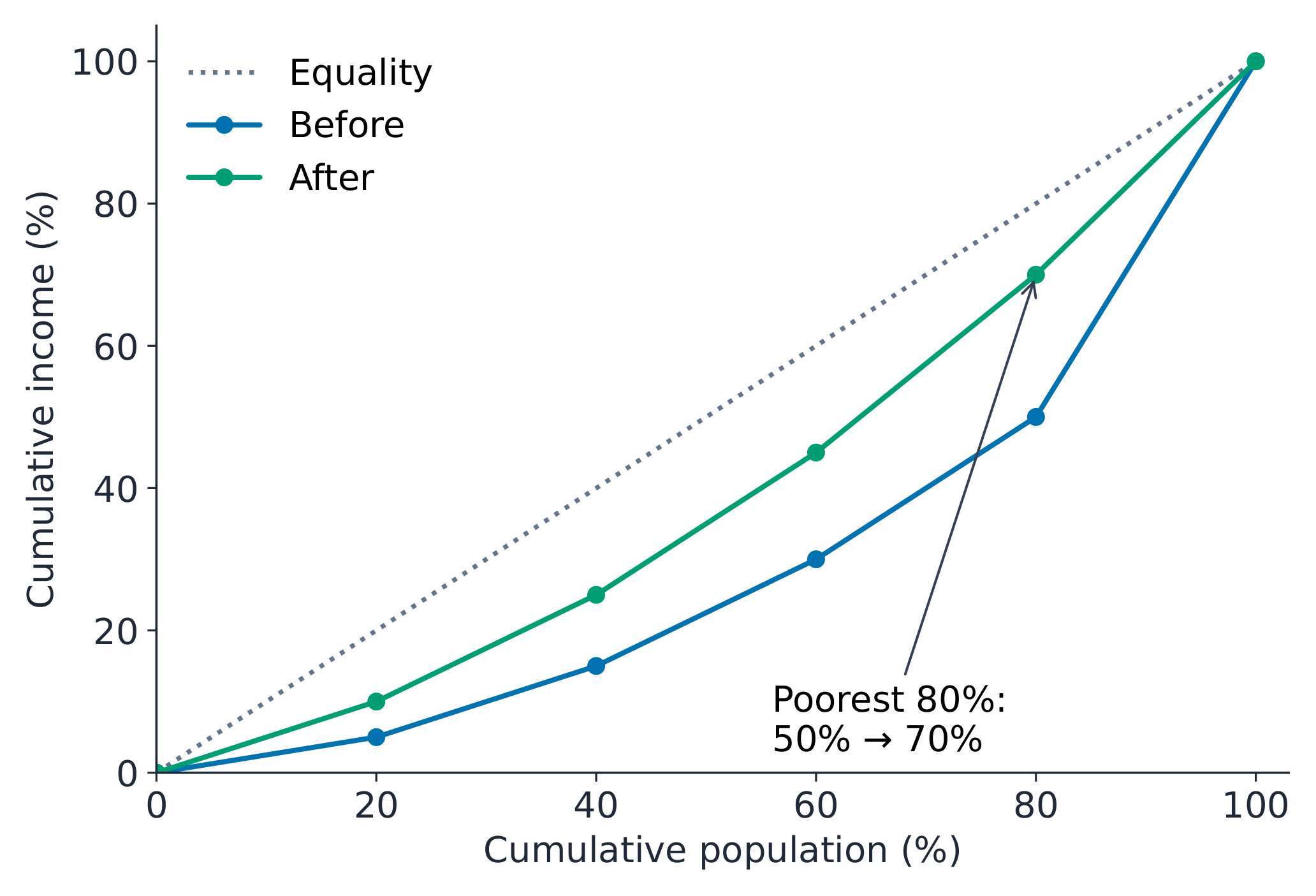
The Lorenz curve 洛伦兹曲线 shows cumulative income share against cumulative population share, ordered from lowest to highest income. The equality line gives every population share the same income share. A curve farther below it indicates more inequality when the curves do not cross. A Gini coefficient 基尼系数 summarizes inequality: zero indicates equality; values closer to one indicate more inequality under the usual nonnegative-income convention. Compare the same population and income definition.
Read complete distributions rather than a photograph
These are illustrative shares for five equally sized groups, ordered by income. The second distribution represents a possible outcome after taxes and transfers, not a forecast that every policy produces it.
| Group, lowest to highest | Before | After |
|---|---|---|
| First fifth | 5% | 10% |
| Second fifth | 10% | 15% |
| Third fifth | 15% | 20% |
| Fourth fifth | 20% | 25% |
| Fifth fifth | 50% | 30% |
Before, the poorest 40% receive 15% of income; after, they receive 25%. The corresponding poorest 80% shares are 50% and 70%. The after curve is everywhere above the before curve except at the endpoints, so the after distribution is less unequal. Do not infer an exact Gini coefficient from only a bottom and top share. AP requires interpreting these measures, not drawing Lorenz curves or calculating Gini coefficients.
Taxes, access and incentives
Human capital 人力资本 includes education and skills. Inheritance, social networks, discrimination, access to finance, mobility and bargaining power can also affect income and wealth. Do not assume pay differences always measure productivity or rank one source as the largest without evidence.
Compare average tax rates
Progressive taxes 累进税 take a higher average share as income rises. For incomes $10,000 and $40,000, taxes $1,000 and $8,000 give average rates 10% and 20%. A proportional 20% tax takes the same average share. A fixed $1,000 levy takes 10% from the lower income but 2.5% from the higher income, making its average burden regressive. A higher absolute tax payment alone does not prove progression, and marginal tax brackets are not rates applied to every dollar of income.
Transfer payments 转移支付 change disposable income without being payment for current production, for example a household cash benefit. Taxes and transfers can alter measured inequality; compare distributions using the same definitions before and after.
The efficiency–equity trade-off 效率与公平权衡 is a possible tension, not a fixed law. Some designs reduce incentives to work or invest. Others improve health, education or access to jobs and may increase both opportunity and productivity. Evaluate a particular policy's incentives, funding and effects.
Measure inequality with a Lorenz curve
A Lorenz curve plots cumulative income against cumulative population; the further it bows from the diagonal, the more unequal — summarised by the Gini coefficient.
| English |
|---|
| income distribution/ˈɪŋkʌm ˌdɪstrɪˈbjuːʃn/ |
| Lorenz curve/ˈlɒrənts kɜːv/ |
| Gini coefficient/ˈdʒiːni ˌkəʊɪˈfɪʃənt/ |
| human capital/ˈhjuːmən ˈkæpɪtl/ |
| progressive taxes/prəˈɡresɪv ˈtæksɪz/ |
| transfer payments/ˈtrænsfɜː ˈpeɪmənts/ |
| efficiency–equity trade-off/ɪˈfɪʃənsi ˈekwɪti treɪd ɒf/ |
6.5
Exam tips
- Identify the third-party effect and the correct private and social curves.
- Calculate DWL over inefficient units; distinguish harm, transfers and fiscal cost.
- Check buyer and seller prices and the quantity actually supplied under a ceiling.
- Distinguish fixed charges from marginal incentives, and zero profit from efficiency.
- Classify goods by rivalry and excludability, not their funding.
- Compare complete income distributions; do not infer Gini from a photo or two shares.
Interactive lessons on this topic
Work through it step by step, with instant-check exercises.