| Enduring Understanding | Learning Objective | Essential Knowledge |
|---|---|---|
PRD-1 | PRD-1.A |
|
Production, Cost, and the Perfect Competition Model
AP Microeconomics · Topic 3
 8:56
8:56
Production, Cost & Perfect Competition
Picture a small bakery with one kitchen and one oven. Hire your first baker and you get thirty extra loaves a day. Hire a second and you get twenty-six more. A…
English narration · English + 中文 subtitles burned in
3.1
The Production Function
Syllabus
Source: College Board AP Course and Exam Description
The production function 生产函数 links inputs to output. In the short run 短期 at least one input (usually capital) is fixed 固定; in the long run 长期 all inputs vary.
- Total product 总产量 is the total output.
- Marginal product 边际产量 (MP) is the extra output from one more unit of a variable input (usually labor): $MP=\dfrac{\Delta\ \text{output}}{\Delta\ \text{labor}}$.
- Average product 平均产量 is output per worker.
As you add workers to fixed capital, MP eventually falls – the law of diminishing marginal returns 边际收益递减法则. With a constant wage and labor as the only variable input, lower MP raises marginal cost. This relationship depends on input prices and the production conditions.

Worked example: one oven and four workers
The oven and technology stay fixed. All workers work equal daily hours. With 0, 1, 2, 3 and 4 workers, total product is 0, 10, 24, 33 and 39 loaves per day. First calculate each extra worker’s contribution, then average output at three workers.
$MP=\Delta TP/\Delta L$ gives 10, 14, 9 and 6 loaves per worker-day. The third worker starts diminishing marginal returns because MP falls from 14 to 9. Total output still rises from 24 to 33: positive but falling MP means less extra output, not falling output. $AP=TP/L=33/3=11$ loaves per worker-day.
Use the production table to choose workers
Use the bakery's production data above. Price is $8 per loaf and wage $60 per worker-day. Labor is the only variable input; the oven's fixed cost is unavoidable today. Choices are zero through four workers.
| Worker added | 1 | 2 | 3 | 4 |
|---|---|---|---|---|
| Extra loaves MP | 10 | 14 | 9 | 6 |
| Extra revenue P×MP | 80 | 112 | 72 | 48 |
| Extra labor cost | 60 | 60 | 60 | 60 |
| Extra profit | 20 | 52 | 12 | −12 |
Money rows are dollars per day. Choose three workers: the third adds $72 revenue for $60 cost; the fourth lowers profit by $12. The first three contribute $84 toward unavoidable fixed cost and profit.
Vocabulary
Train
| English |
|---|
| production function/prəˈdʌkʃn ˈfʌŋkʃn/ |
| short run/ʃɔːt rʌn/ |
| fixed/fɪkst/ |
| long run/lɒŋ rʌn/ |
| Total product/ˈtəʊtl ˈprɒdʌkt/ |
| Marginal product/ˈmɑːdʒɪnl ˈprɒdʌkt/ |
| Average product/ˈævrɪdʒ ˈprɒdʌkt/ |
| law of diminishing marginal returns/lɔː ɒv dɪˈmɪnɪʃɪŋ ˈmɑːdʒɪnl rɪˈtɜːnz/ |
3.2
Short-Run Production Costs
Syllabus
| Enduring Understanding | Learning Objective | Essential Knowledge |
|---|---|---|
PRD-1 | PRD-1.A |
|
Source: College Board AP Course and Exam Description
Costs split into fixed and variable:
- Fixed cost 固定成本 (FC) does not change with output (rent on the factory).
- Variable cost 可变成本 (VC) rises with output (materials, labor).
- Total cost 总成本 $TC=FC+VC$.
The per-unit costs matter most:
- Average fixed cost $AFC=FC/Q$ falls continuously (spreading fixed cost).
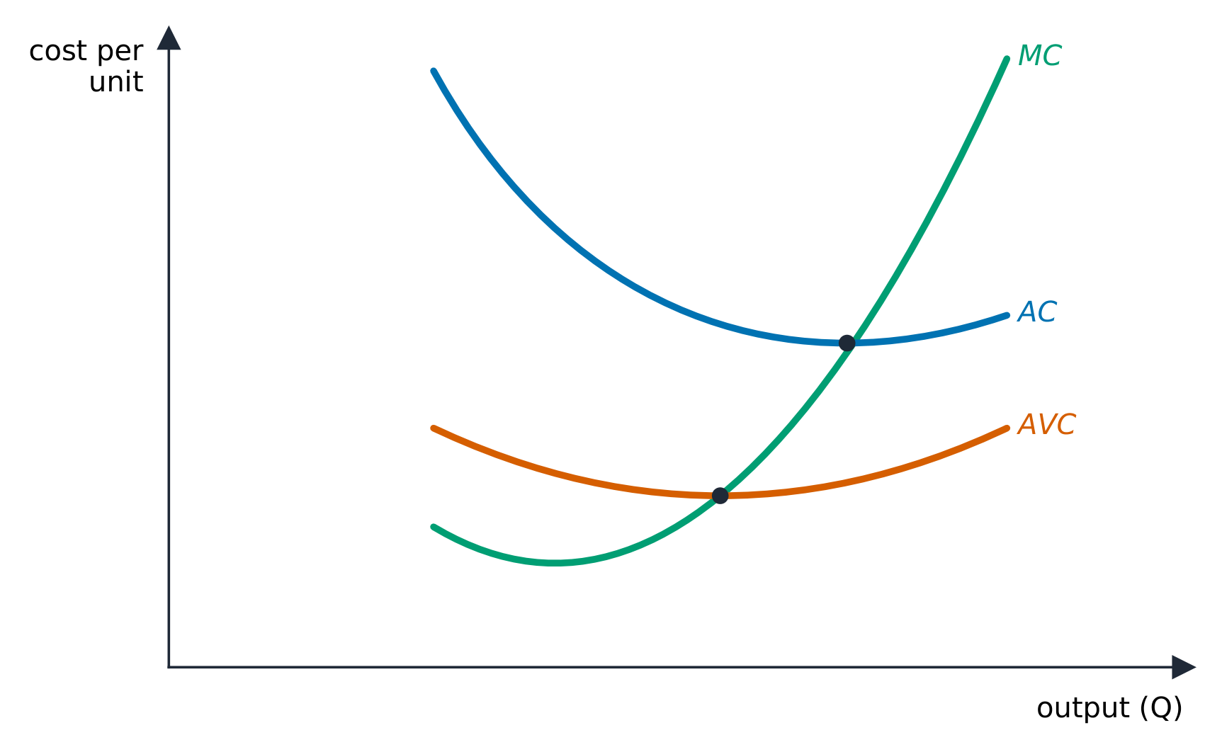
- Average variable cost $AVC=VC/Q$ and average total cost $ATC=TC/Q$ commonly have U-shaped curves in standard short-run diagrams; the shapes depend on production conditions.
- Marginal cost 边际成本 $MC=\dfrac{\Delta TC}{\Delta Q}$ is the cost of one more unit.
With constant wage $w$ and labor as the only variable input, $MC=w/MP$: a lower MP raises MC. This is an inverse numerical relationship, not a literal reflection of graphs. MC cuts both AVC and ATC at their minimum points in the standard smooth cost model: when marginal is below average, average falls; when above, average rises.
Worked example. A firm has fixed cost $FC=\$100$. At $Q=10$ its total cost is $\$300$, so variable cost is $\$200$: then $ATC=\tfrac{300}{10}=\$30$, $AVC=\tfrac{200}{10}=\$20$, and $AFC=\tfrac{100}{10}=\$10$ (note $AFC+AVC=ATC$). If raising output to $Q=11$ pushes total cost to $\$325$, the marginal cost of that $11$th unit is $\dfrac{\Delta TC}{\Delta Q}=\dfrac{325-300}{1}=\$25$.
Explain the cost change
In the cost example, the eleventh unit costs $25, below the previous ATC of $30. New $ATC=TC/Q=325/11\approx\$29.55$ per unit. At zero output the $100 fixed cost remains, but average costs are undefined because their denominator is zero.
For the bakery above, assume each worker costs $60 per day and labor is the only variable input. The second, third and fourth workers add 14, 9 and 6 loaves. Their extra cost per loaf is $MC=\Delta VC/\Delta Q=60/14\approx\$4.29$, $MC=60/9\approx\$6.67$, and $MC=60/6=\$10$. This shows why diminishing marginal returns raises MC when wage is unchanged.
If fixed rent alone rises by $50, FC rises and ATC rises by $50/Q$ dollars per unit. AVC and MC stay unchanged: an extra unit does not add rent. If wage rises while productivity stays unchanged, variable cost, AVC, ATC and MC rise at positive output. Cost curves respond to the affected input; do not shift every curve automatically.
Explore
Explore the U-shaped cost curves
Compare marginal and average costs as output changes; marginal cost below average pulls the average down, and marginal cost above average pushes it up.
Vocabulary
Train
| English |
|---|
| Fixed cost/fɪkst kɒst/ |
| Variable cost/ˈveərɪəbl kɒst/ |
| Total cost/ˈtəʊtl kɒst/ |
| Marginal cost/ˈmɑːdʒɪnl kɒst/ |
3.3
Long-Run Production Costs
Syllabus
| Enduring Understanding | Learning Objective | Essential Knowledge |
|---|---|---|
PRD-1 | PRD-1.A |
|
Source: College Board AP Course and Exam Description
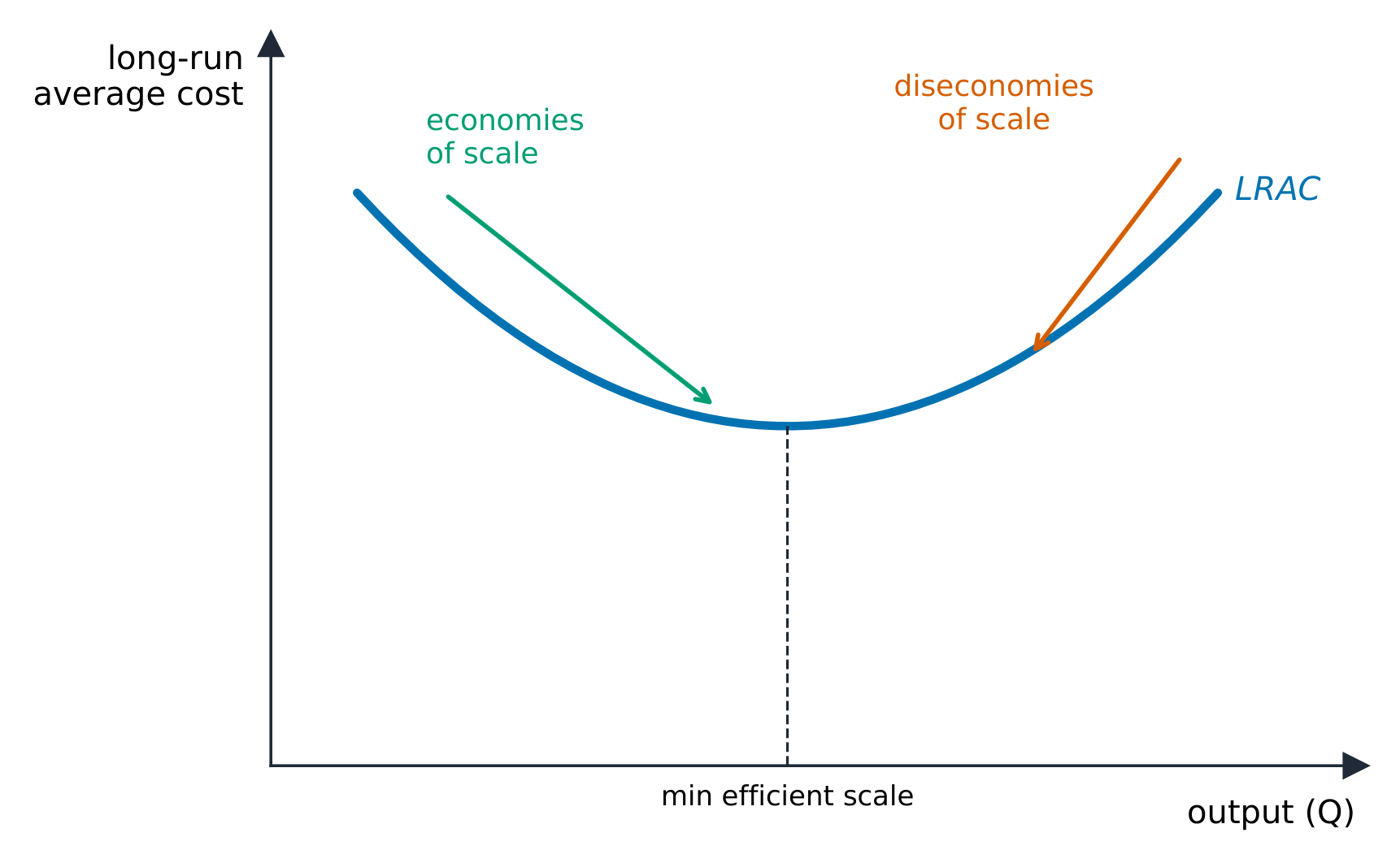
In the long run all inputs – including plant size – can change, and all costs become variable. The long-run average total cost (LRATC) curve shows the lowest average cost attainable across plant choices:
- Economies of scale 规模经济: LRATC falls as output grows (bulk buying, specialization).
- Constant-cost range: LRATC is flat. At unchanged input prices, constant returns to scale can produce this pattern.
- Diseconomies of scale 规模不经济: LRATC rises (a firm too big to manage well).
Exam skill: know that "diminishing returns" is a short-run idea (one fixed input) while "economies of scale" is a long-run idea (all inputs vary) – examiners test the distinction.
Worked example: calculate before classifying
Two long-run plans can change all inputs. Plan A produces 40 units at total cost $600; plan B produces 60 at total cost $1080. Does higher total cost alone establish diseconomies?
$LRATC=TC/Q=600/40=\$15$ per unit for A; $LRATC=1080/60=\$18$ per unit for B. Rising average cost establishes diseconomies over this output range. Total cost can rise while average cost falls, so total cost alone is insufficient.
Physical returns to scale compares output after all inputs increase proportionately, with technology fixed. If every input doubles, more than double output means increasing returns, exactly double means constant returns, and less than double means decreasing returns. At unchanged input prices, increasing returns can lower average cost; input-price changes also affect cost. This differs from adding labor while holding an oven fixed.
Minimum efficient scale 最小有效规模 is the smallest output at minimum LRATC. When this scale is large relative to market demand, fewer firms can operate at that scale, helping explain market concentration. It does not by itself prove monopoly.
Vocabulary
Train
| English |
|---|
| Economies of scale/ɪˈkɒnəmiz ɒv skeɪl/ |
| Diseconomies of scale/ˌdɪsɪˈkɒnəmiz ɒv skeɪl/ |
| Minimum efficient scale/ˈmɪnɪməm ɪˈfɪʃənt skeɪl/ |
3.4
Types of Profit
Syllabus
| Enduring Understanding | Learning Objective | Essential Knowledge |
|---|---|---|
CBA-2 | CBA-2.C |
|
Source: College Board AP Course and Exam Description
Economists count all opportunity costs, including the owner's. Explicit costs 显性成本 are out-of-pocket payments; implicit costs 隐性成本 are the opportunity costs of owner-supplied resources, such as forgone salary and interest.
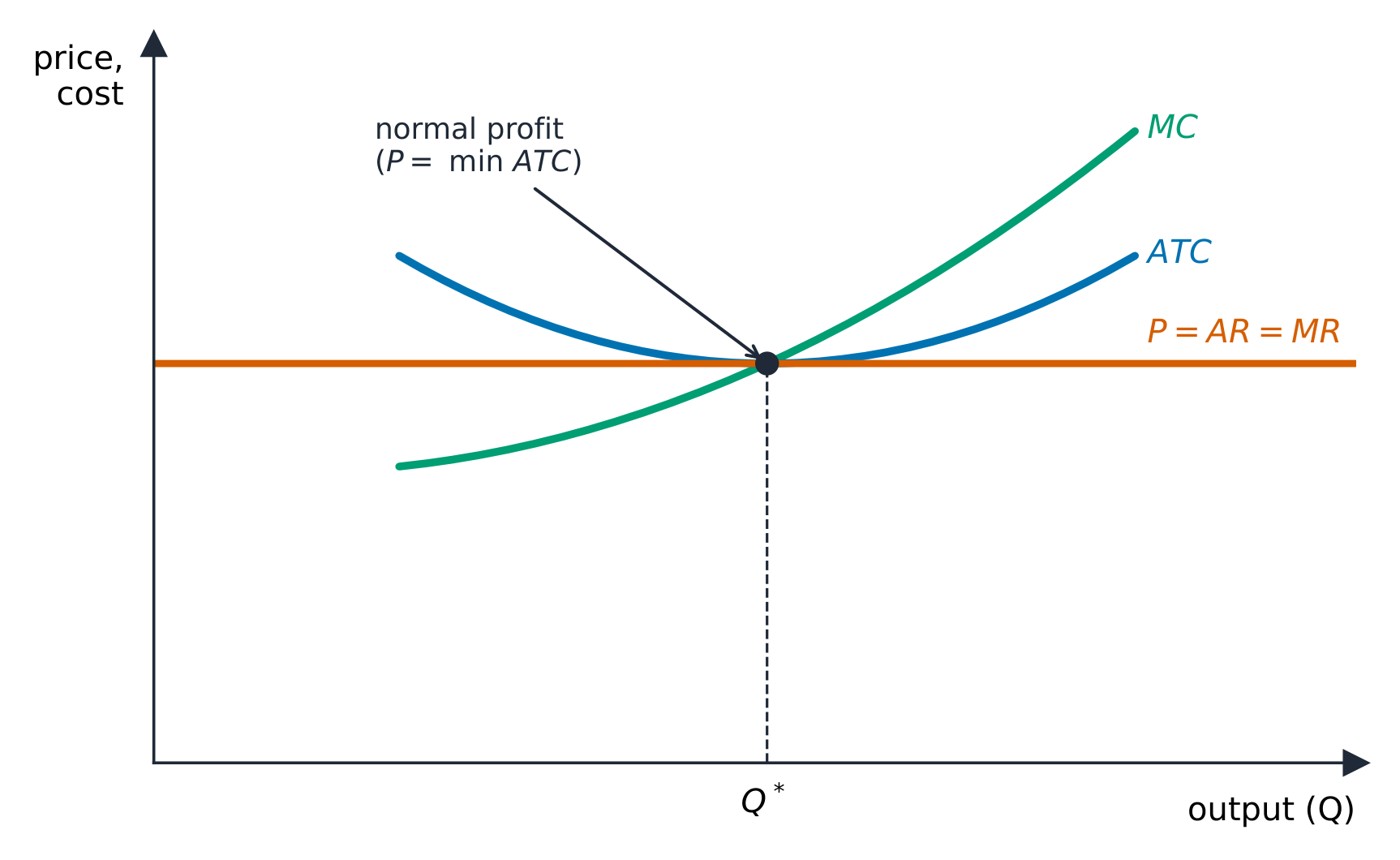
Accounting profit 会计利润 is revenue minus explicit costs. Economic profit 经济利润 also subtracts implicit costs. Normal profit 正常利润 means zero economic profit: every opportunity cost is covered. It can include positive accounting profit and income for the owner.
Worked example: one year's shop accounts
Revenue is $200,000 and payments for rent, wages and materials are $120,000. The owner gives up a $70,000 salary and $5,000 interest on savings invested in the shop. Treat these as all relevant costs over the same year. Calculate the two profits before reading the answers.
Accounting profit $=TR-EC=200,000-120,000=\$80,000$.
Implicit costs $=70,000+5,000=\$75,000$.
Economic profit $=TR-EC-IC=200,000-120,000-75,000=\$5,000$.
On these complete data, the business pays more than its next-best alternative. Positive accounting profit alone cannot establish that conclusion: with $90,000 implicit costs, the same accounting profit would imply an economic loss of $10,000. Short-run operation and long-run exit still require their own comparisons below.
Vocabulary
Train
| English |
|---|
| Explicit costs/ekˈsplɪsɪt kɒsts/ |
| implicit costs/ɪmˈplɪsɪt kɒsts/ |
| Accounting profit/əˈkaʊntɪŋ ˈprɒfɪt/ |
| Economic profit/ˌiːkəˈnɒmɪk ˈprɒfɪt/ |
| normal profit/ˈnɔːml ˈprɒfɪt/ |
3.5
Profit Maximization
Syllabus
| Enduring Understanding | Learning Objective | Essential Knowledge |
|---|---|---|
CBA-2 | CBA-2.D |
|
Source: College Board AP Course and Exam Description
For a smooth interior optimum, use $MR=MC$ with MC crossing MR from below. Compare feasible total profits and shutdown too. With discrete output, equality may never occur.
Worked example: choose the best operating output
A price-taking firm can sell at $8 per unit. All costs are economic costs. Its unavoidable fixed cost this period is $32. For continuous output $q$, the cost model is:
$$TC=32+2q+\tfrac12q^2,\qquad VC=2q+\tfrac12q^2,\qquad MC=2+q.$$
This simple numerical model has $AVC=2+\tfrac12q$, rising for positive output, rather than the U-shaped AVC in the earlier schematic. The marginal-versus-average logic still applies.
A price taker has $MR=P=8$. Why use the marginal rule? Additional units before the crossing add more revenue than cost; beyond it, extra cost exceeds extra revenue.
$$MR=MC$$
$$8=2+q$$
$$q=8-2=6\text{ units}.$$
Revenue is $TR=Pq=8(6)=\$48$.
Variable cost is $VC=2q+\tfrac12q^2=2(6)+\tfrac12(6)^2=\$30$.
Economic profit is $\pi=TR-FC-VC=48-32-30=-\$14$. The best operating output makes a loss; that does not yet prove shutdown is preferable.
Discrete choices: compare all feasible profits
A different firm sells indivisible units at $8 each. Its complete feasible outputs are 0, 1, 2, 3 and 4. Total costs are respectively $10, $14, $19, $26 and $36. Calculate revenue and profit at each output.
$TR=Pq$ gives $0, $8, $16, $24 and $32. $\pi=TR-TC$ gives −$10, −$6, −$3, −$2 and −$4. Choose three units. The third unit adds $8 revenue and $7 cost; the fourth adds $8 revenue and $10 cost. No MR=MC equality is needed, and three units beat zero output despite making a loss.
3.6
Deciding to Produce, Enter, or Exit
Syllabus
| Enduring Understanding | Learning Objective | Essential Knowledge |
|---|---|---|
PRD-2 | PRD-2.A |
|
Source: College Board AP Course and Exam Description
For a price taker, compare price with average variable cost at its best positive operating output. If $P>AVC$, revenue covers variable cost and contributes toward fixed cost; operating is preferable to shutdown when fixed cost is unavoidable. If $P
Worked decision: minimize the short-run loss
For the continuous-output firm above, operating at six units gives a $14 loss. Shutting down makes output and variable cost zero, but leaves $32 fixed cost: $\pi=-FC=-\$32$. Operating reduces the loss by $18 because $TR-VC=48-30=\$18$ contributes to fixed cost.
At this output, $AVC=VC/q=30/6=\$5$ and $ATC=TC/q=62/6\approx\$10.33$. Price $8 is below ATC but above AVC. A loss and a decision to operate can therefore coexist.
If price instead falls to $1, every positive output has $TR=q
For a separate boundary case, suppose the best positive output is five units at price $4, with VC$20 and unavoidable FC$10. $TR=Pq=4(5)=\$20=VC$; operating profit is $\pi=20-20-10=-\$10$, equal to shutdown profit $\pi=-FC=-\$10$.
Entry 进入 and exit 退出 are long-run decisions. When commitments can change, expected continuing economic losses encourage exit and expected positive economic profit encourages entry if entry is free. A temporary loss does not alone establish that leaving the industry is best. Normal profit permits a firm to stay: its next-best resource uses are already compensated.
Vocabulary
Train
| English |
|---|
| entry/ˈentri/ |
| exit/ˈeɡzɪt/ |
3.7
Perfect Competition
Syllabus
| Enduring Understanding | Learning Objective | Essential Knowledge |
|---|---|---|
PRD-3 | PRD-3.A |
|
Source: College Board AP Course and Exam Description
A perfectly competitive 完全竞争 market has many small firms, identical products, free entry and exit, and perfect information. Each firm is a price taker 价格接受者. Its horizontal demand curve is at the market price, with $P=MR=AR$. The whole market still has downward-sloping demand.
If identical products remain available from other sellers at $12, one tiny seller charging $13 sells nothing and earns zero revenue. This conclusion depends on the ideal market assumptions; it is not a claim that any real business raising price loses all customers.
Read the market and firm graphs separately
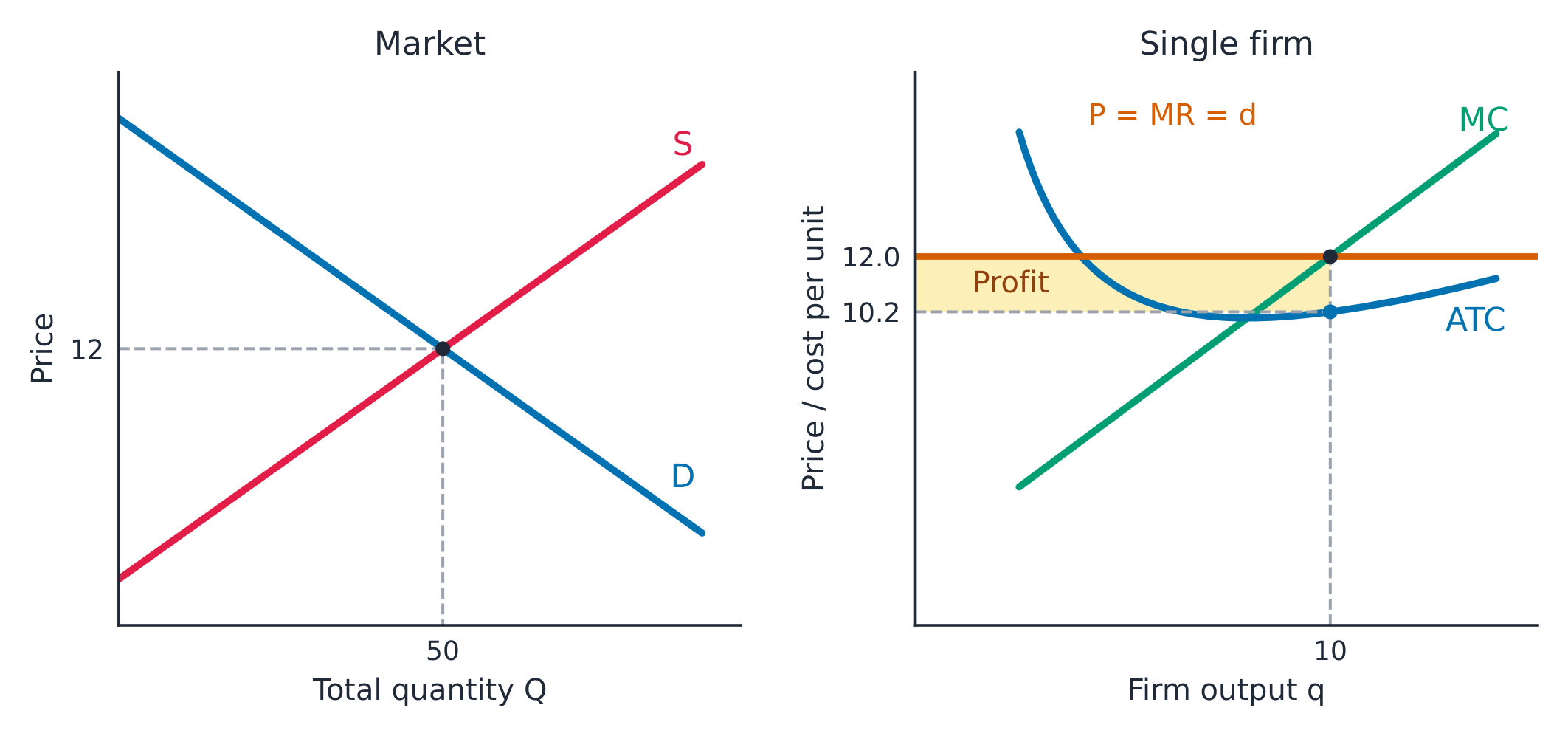
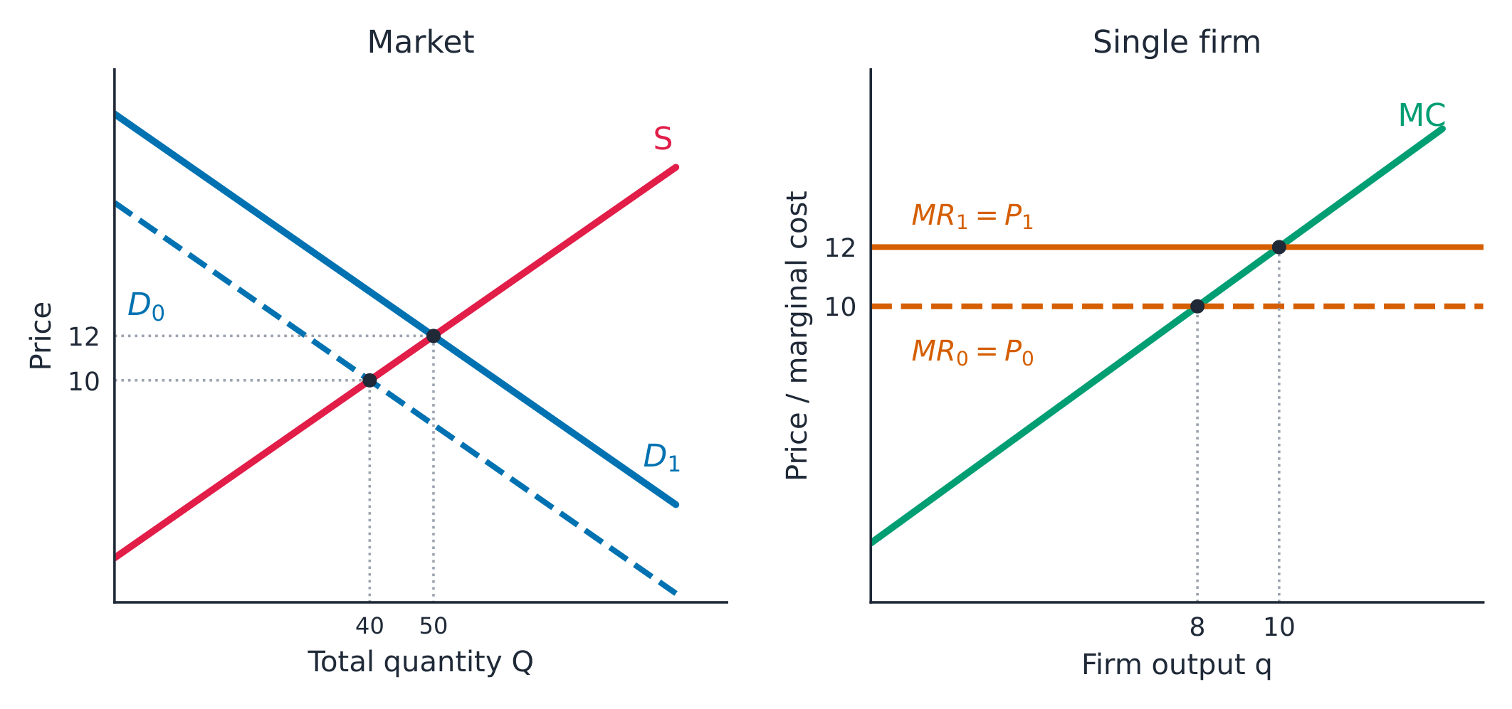
The market shown has inverse demand $P=22-0.2Q$ and supply $P=2+0.2Q$. Equality gives market quantity $Q=50$ and price $P=12$. Market quantity $Q$ aggregates firms; individual output $q$ uses a separate axis.
For the continuous-output firm, $MC=2+q=12$ gives $q=10$. $TC=32+2(10)+\tfrac12(10)^2=\$102$, so $ATC=TC/q=102/10=\$10.20$. Profit is $\pi=(P-ATC)q=(12-10.2)10=\$18$. Read ATC at ten units, not at its minimum eight-unit output. The native curves come from this same cost model; MC is already rising throughout its positive-output range.
One firm can earn profit, normal profit or a loss
With the same cost model, price $12 gives $q=10$, TR$120, TC$102 and profit$18. Price $10 gives $q=8$, TR$80, TC$80 and zero economic profit. Price $8 gives $q=6$, TR$48, TC$62 and loss$14, with operation still preferable to shutdown. These are separate market-price cases, not choices the price-taking firm sets itself.
Demand shock and long-run entry
Suppose the market initially has demand $P=18-0.2Q$ and supply $P=2+0.2Q$, giving $Q=40$ and $P=10$. The typical firm produces eight units at minimum ATC and earns normal profit. A permanent increase in demand to $P=22-0.2Q$ gives short-run $Q=50$ and $P=12$. Market demand shifts right; the firm's horizontal MR line rises. Its cost curves stay unchanged unless input costs or productivity change. Firm output rises from eight to ten and profit becomes $18.
Entry in a constant-cost industry
In a constant-cost industry 成本不变行业, new firms can enter without changing input prices or firms' cost curves. Profit attracts entry, market supply shifts right, and long-run price returns to the unchanged minimum ATC of $10. With the higher demand, market quantity becomes $Q=(22-10)/0.2=60$. Each typical firm returns to eight units. More firms can raise total market output while each incumbent makes less than at the short-run peak. The model treats entry continuously; these graph quantities are illustrative scales, not a literal count of firms.
After a demand fall, continuing losses encourage exit and supply shifts left. Adjustment takes time and relies on the entry/exit assumptions.
Industry costs can change as the market expands
Return to an initial price of $10. Suppose higher demand and industry expansion leave the new minimum average cost at $10 in industry A, $11 in B and $9 in C. With free entry and comparable firms, zero-economic-profit long-run prices are respectively $10, $11 and $9. A is constant-cost. B is an increasing-cost industry 成本递增行业; C is a decreasing-cost industry 成本递减行业. Scarcer inputs can raise input prices as an industry expands; external economies can lower costs. This is different from a single firm's internal economies or diseconomies of scale. Do not promise that price always returns to its original level.
Efficiency: two tests
Productively efficient 生产效率 output is at minimum ATC. Allocatively efficient 配置效率 output satisfies $P=MC$ when private marginal costs and benefits equal social ones. In the competitive long-run benchmark, operating firms satisfy $P=MC=\min ATC$ and earn normal profit. A short-run price-taking firm can satisfy $P=MC$ while producing away from minimum ATC.
Draw separate market and firm axes, label their different quantities, show the relevant demand/supply or MR/cost curves, and mark the profit/loss rectangle before explaining entry or exit. The 2024 Set1 soybean task explicitly requires this graph sequence; the 2024 Set2 production task requires output-based AFC/MC calculations and numerical diminishing-returns and scale explanations.
Explore
The market price before the firm’s decision
Market demand and supply determine the price that a competitive firm takes as given. The separate firm diagram in the lesson explains its output and profit; this activity displays the market.
Vocabulary
Train
| English |
|---|
| perfectly competitive/ˈpɜːfektlɪ kəmˈpetɪtɪv/ |
| price taker/praɪs ˈteɪkə/ |
| allocatively efficient/ˈæləkətɪvli ɪˈfɪʃənt/ |
| productively efficient/prəˈdʌktɪvli ɪˈfɪʃənt/ |
| constant-cost industry/ˈkɒnstənt kɒst ˈɪndʌstri/ |
| increasing-cost industry/ɪnˈkriːsɪŋ kɒst ˈɪndʌstri/ |
| decreasing-cost industry/ˈdiːkriːsɪŋ kɒst ˈɪndʌstri/ |
3.7
Exam tips
- Show the formula, substitute the data, and give units. Separate total, average and marginal values.
- Label market and firm graphs separately; mark output, price and the profit or loss rectangle.
- State which inputs are fixed before explaining diminishing returns or returns to scale. Check shutdown separately from the best operating output.
Interactive lessons on this topic
Work through it step by step, with instant-check exercises.