| Enduring Understanding | Learning Objective | Essential Knowledge |
|---|---|---|
MKT-3 | MKT-3.A |
|
MKT-3.B |
|
Supply and Demand
AP Microeconomics · Topic 2
 10:39
10:39
Supply and Demand
Why does a cup of coffee cost what it costs? Nobody decided it. There is no committee and no official price list. There are only buyers, who want more when it…
English narration · English + 中文 subtitles burned in
2.1
Demand

Syllabus
Source: College Board AP Course and Exam Description
Well-defined property rights 产权 support exchange: owners can use, exclude others from, and trade their resources. Within that framework, the two forces are demand and supply.
Demand 需求 is the relationship between the price of a good and the quantity buyers are willing and able to buy. The law of demand 需求定律 says that, with other conditions held constant, price and quantity demanded move in opposite directions, so the demand curve slopes downward. Two reasons: the substitution effect 替代效应 (when a good gets pricier, buyers switch to alternatives) and the income effect 收入效应 (a higher price shrinks real purchasing power).
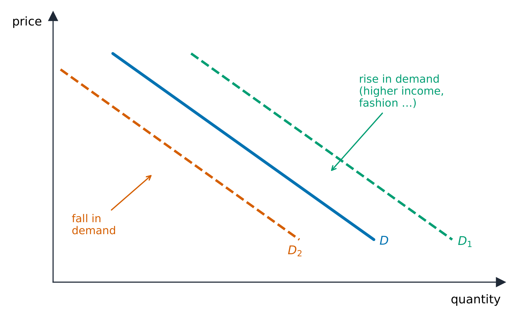
Distinguish a change in quantity demanded (a move along the curve, caused only by the good's own price) from a change in demand (a shift of the whole curve). Demand shifts with the determinants 决定因素, remembered as TRIBE:
- Tastes/preferences,
- Related goods – a rise in the price of a substitute 替代品 raises demand; a rise in the price of a complement 互补品 lowers it,
- Income – for a normal good 正常商品 more income raises demand; for an inferior good 低档商品 it lowers it,
- Buyers (number of consumers),
- Expectations of future price or income.
The market demand curve is the horizontal summation 水平相加 of every individual buyer's demand curve – at each price, add up the quantities all buyers want. That is why more buyers (the B above) shifts the whole market curve to the right.
Explore
Shift demand and watch price and quantity
The demand curve slopes down: lower price, more wanted. A change in income, tastes or related-good prices shifts the whole curve, moving the equilibrium.
Vocabulary
Train
| English |
|---|
| property rights/ˈprɒpəti raɪts/ |
| Demand/dɪˈmænd/ |
| law of demand/lɔː ɒv dɪˈmænd/ |
| substitution effect/ˌsʌbstɪˈtjuːʃn ɪˈfekt/ |
| income effect/ˈɪŋkʌm ɪˈfekt/ |
| determinants/dɪˈtɜːmɪnənts/ |
| substitute/ˈsʌbstɪtjuːt/ |
| complement/ˈkɒmplɪmənt/ |
| normal good/ˈnɔːml ɡʊd/ |
| inferior good/ɪnˈfɪərɪə ɡʊd/ |
| horizontal summation/ˌhɒrɪˈzɒntl sʌˈmeɪʃn/ |
2.2
Supply
Syllabus
| Enduring Understanding | Learning Objective | Essential Knowledge |
|---|---|---|
MKT-3 | MKT-3.C |
|
MKT-3.D |
|
Source: College Board AP Course and Exam Description
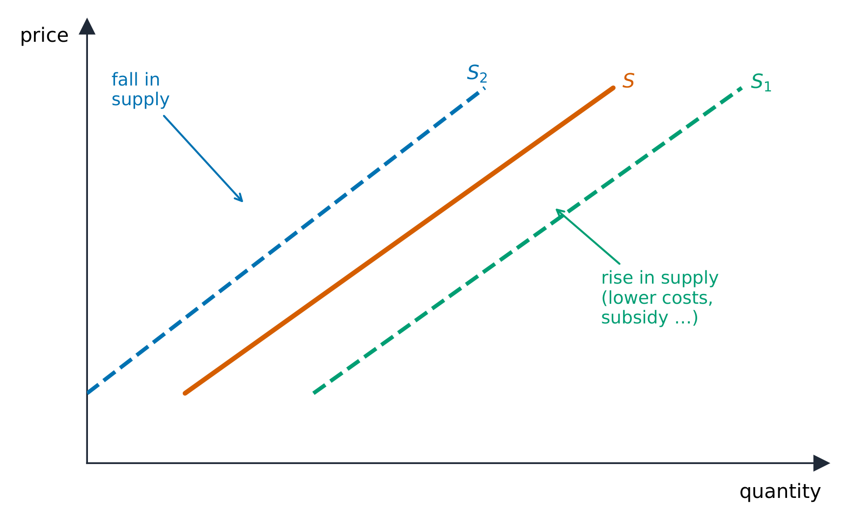
Supply 供给 is the relationship between price and the quantity sellers will offer. The law of supply 供给定律: with other conditions held constant, price and quantity supplied move in the same direction, so the supply curve slopes upward (higher prices cover higher marginal costs and reward more output).
Again separate a change in quantity supplied (movement along the curve, from the good's own price) from a change in supply (a shift). Supply shifts with input prices, technology, taxes and subsidies 补贴, prices of other goods a firm could make, number of sellers, and expectations. Just like demand, the market supply curve is the horizontal sum of individual firms' supply curves – add the quantities all firms offer at each price – so more sellers shifts market supply to the right.
Exam skill: on the free-response section you must draw correctly labeled supply-and-demand graphs and shift the right curve in the right direction – decide first whether the event changes an "own price" (move along) or a determinant (shift).
Vocabulary
Train
| English |
|---|
| Supply/səˈplaɪ/ |
| law of supply/lɔː ɒv səˈplaɪ/ |
| subsidies/ˈsʌbsɪdiz/ |
2.3
Price Elasticity of Demand
Syllabus
| Enduring Understanding | Learning Objective | Essential Knowledge |
|---|---|---|
MKT-3 | MKT-3.E |
|
Source: College Board AP Course and Exam Description
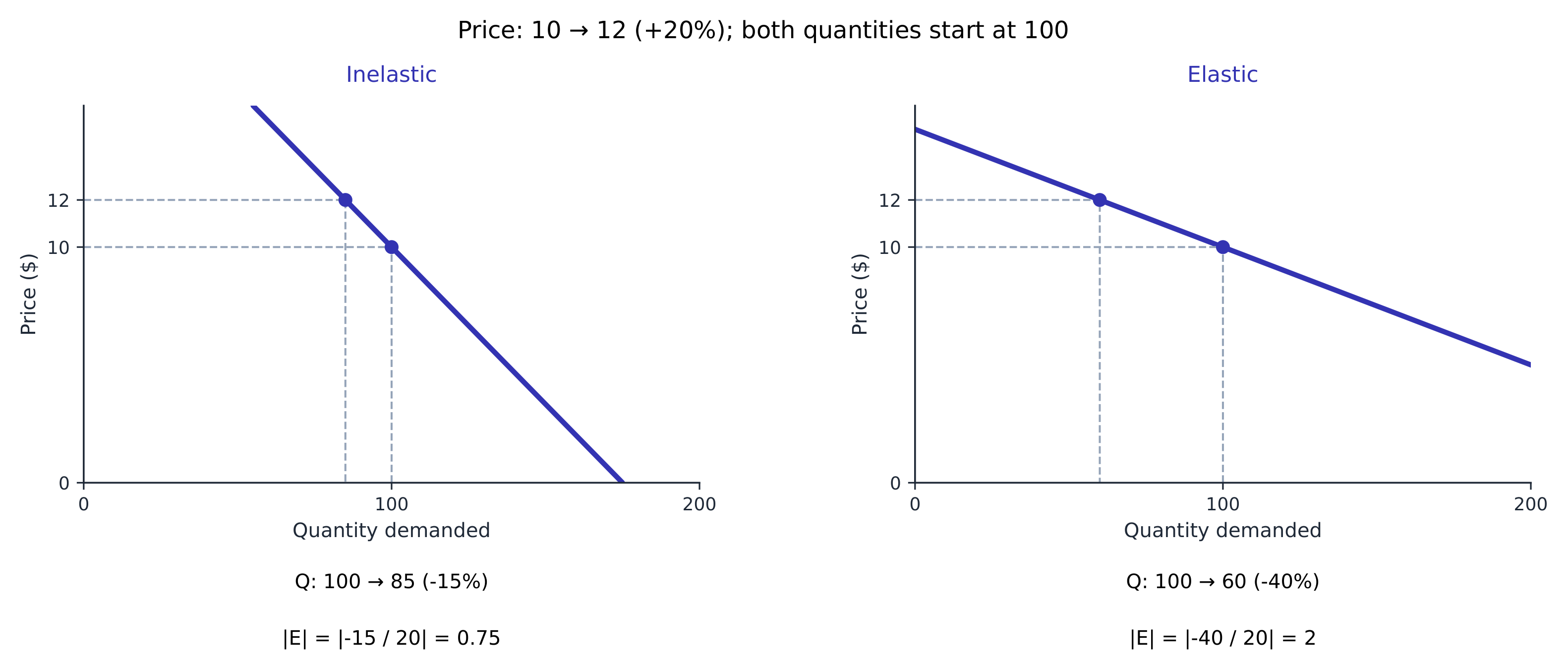
Price elasticity of demand 需求价格弹性 measures how responsive quantity demanded is to a price change:
$$E_d=\left|\frac{\%\ \Delta\ \text{quantity demanded}}{\%\ \Delta\ \text{price}}\right|.$$
- $E_d>1$: elastic 富有弹性 (quantity responds strongly);
- $E_d<1$: inelastic 缺乏弹性 (quantity barely responds);
- $E_d=1$: unit elastic.
Demand is more elastic when there are more substitutes, the good is a luxury, it takes a large share of income, or buyers have more time to adjust. Elasticity links to total revenue 总收入 ($P\times Q$): if demand is elastic, a price cut raises revenue; if inelastic, a price cut lowers it. Elasticity compares percentage changes, not slope alone. Along a straight-line demand curve with positive intercepts, elasticity falls as you move down (elastic on top, inelastic at the bottom).
Worked example (percentage changes measured from the initial values). A price rise from $\$10$ to $\$12$ (a $+20\%$ change) cuts quantity demanded from $100$ to $85$ (a $-15\%$ change). Then $E_d=\left|\dfrac{-15\%}{20\%}\right|=0.75<1$, so demand is inelastic. Because it is inelastic, the price rise raises total revenue: from $\$10\times100=\$1000$ to $\$12\times85=\$1020$.
Explore
Stretch price and measure elasticity
Price elasticity of demand compares percentage changes in quantity demanded and price. Calculate the ratio; slope alone does not establish elasticity, which varies along a straight-line demand curve.
Vocabulary
Train
| English |
|---|
| Price elasticity of demand/praɪs ɪlæˈstɪsɪti ɒv dɪˈmænd/ |
| elastic/ɪˈlæstɪk/ |
| inelastic/ɪnɪˈlæstɪk/ |
| total revenue/ˈtəʊtl ˈrevənjuː/ |
2.4
Price Elasticity of Supply
Syllabus
| Enduring Understanding | Learning Objective | Essential Knowledge |
|---|---|---|
MKT-3 | MKT-3.E |
|
Source: College Board AP Course and Exam Description
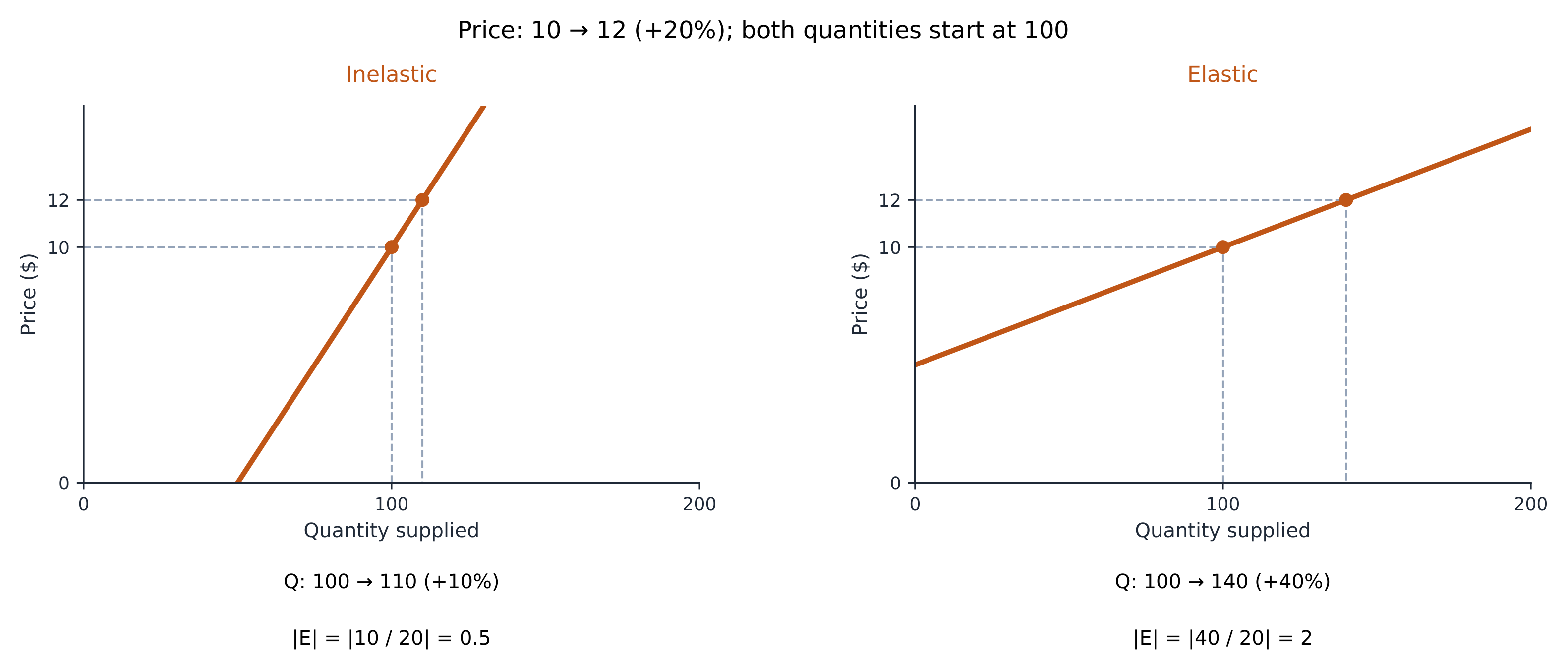
Price elasticity of supply 供给价格弹性, $E_s=\dfrac{\%\ \Delta\ Q_s}{\%\ \Delta\ P}$, measures how responsive sellers are. Supply is more elastic when firms can adjust output easily – spare capacity, storable goods, more time usually gives firms more ways to adjust output; it does not guarantee a particular elasticity.
Worked supply comparison. Both firms start at price $\$10$ and quantity $100$. Price rises to $\$12$, a $20\%$ rise from the initial price. Firm A increases supply to $110$ units, a $10\%$ rise; firm B to $140$, a $40\%$ rise. Using these initial-value percentage changes:
$$E_{s,A}=\frac{\%\Delta Q_s}{\%\Delta P}=\frac{10}{20}=0.5,\qquad E_{s,B}=\frac{40}{20}=2.$$
Firm A has inelastic supply; firm B has elastic supply. Horizontal supply is perfectly elastic; vertical supply is perfectly inelastic.
Vocabulary
Train
| English |
|---|
| Price elasticity of supply/praɪs ɪlæˈstɪsɪti ɒv səˈplaɪ/ |
2.5
Other Elasticities
Syllabus
| Enduring Understanding | Learning Objective | Essential Knowledge |
|---|---|---|
MKT-3 | MKT-3.E |
|
Source: College Board AP Course and Exam Description
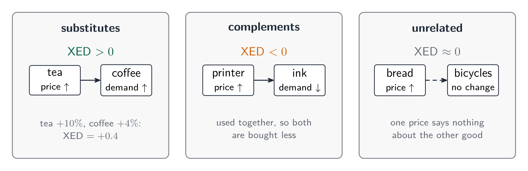
- Cross-price elasticity 交叉价格弹性 $=\dfrac{\%\ \Delta\ Q_x}{\%\ \Delta\ P_y}$: positive for substitutes, negative for complements – the sign tells you the relationship.
- Income elasticity 收入弹性 $=\dfrac{\%\ \Delta\ Q}{\%\ \Delta\ \text{income}}$: positive for normal goods (and $>1$ for luxuries), negative for inferior goods.
Worked example. When the price of coffee rises $10\%$, the quantity of tea demanded rises $6\%$: cross-price elasticity $=\dfrac{+6\%}{+10\%}=+0.6$. The positive sign confirms coffee and tea are substitutes. If instead a $5\%$ rise in incomes raised restaurant-meal demand $10\%$, income elasticity $=\dfrac{10\%}{5\%}=+2$ – a normal good, and a luxury since it exceeds $1$.
Further practice and answers. Printer price rises $10\%$ and ink quantity demanded falls $4\%$: $E_{ink,printer}=\frac{-4}{10}=-0.4$, so they are complements. Income rises $10\%$ and bus-ticket quantity demanded falls $5\%$: $E_Y=\frac{-5}{10}=-0.5$, so bus travel is an inferior good in this example. Hold other determinants constant.
Official application: AP 2024 Set 1, Q1(e). Quinoa price rises $25\%$, its quantity demanded falls $5\%$, and tofu quantity demanded rises $10\%$. Own-price elasticity magnitude is $|E_d|=|{-5}/{25}|=0.2$, so quinoa demand is inelastic. Cross-price elasticity is $E_{tofu,quinoa}=10/25=+0.4$, so the goods are substitutes. Neither value establishes whether tofu is normal or inferior; that requires an income change.
Exam skill: you are expected to compute an elasticity, classify it, and read a sign as evidence of substitute/complement or normal/inferior.
Vocabulary
Train
| English |
|---|
| Cross-price elasticity/krɒs praɪs ɪlæˈstɪsɪti/ |
| Income elasticity/ˈɪŋkʌm ɪlæˈstɪsɪti/ |
2.6
Market Equilibrium, Consumer Surplus, and Producer Surplus
Syllabus
| Enduring Understanding | Learning Objective | Essential Knowledge |
|---|---|---|
MKT-4 | MKT-4.A |
|
Source: College Board AP Course and Exam Description
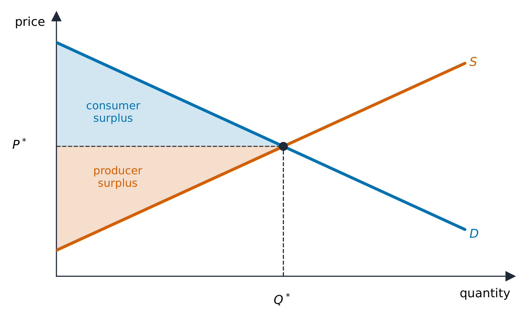
Equilibrium 均衡 is where supply meets demand: the equilibrium price clears the market, so quantity demanded equals quantity supplied and there is no shortage or surplus.
- Consumer surplus 消费者剩余 is the area below the demand curve and above the price – the gap between what buyers would pay and what they do pay.
- Producer surplus 生产者剩余 is the area above the supply curve and below the price – the gap between the price and sellers' minimum acceptable price.
- Their sum is total surplus 总剩余, and a competitive equilibrium maximizes it when there are no market failures. Private benefits and costs must reflect social benefits and costs for this equilibrium to be allocatively efficient 配置有效率.

Worked market used below. Demand is $P_D=20-Q$ and supply is $P_S=2+Q$, with price in dollars and quantity in units. Equilibrium requires equal demand and supply prices:
$$P_D=P_S,\quad20-Q=2+Q,\quad Q^*=9,\quad P^*=\$11.$$
For these straight-line curves, use triangle areas:
$$CS=\tfrac12 Q^*(P_{D,0}-P^*)=\tfrac12(9)(20-11)=\$40.50.$$
$$PS=\tfrac12 Q^*(P^*-P_{S,0})=\tfrac12(9)(11-2)=\$40.50.$$
$$TS=CS+PS=\$81.$$
Assume no external costs or benefits.
Explore
See consumer and producer surplus
At equilibrium the market clears. The gap between what buyers would pay and the price is consumer surplus; the gap above sellers' costs is producer surplus.
Vocabulary
Train
| English |
|---|
| Equilibrium/ˌiːkwɪˈlɪbrɪəm/ |
| Consumer surplus/kənˈsuːmə ˈsɜːpləs/ |
| Producer surplus/prəˈdjuːsə ˈsɜːpləs/ |
| total surplus/ˈtəʊtl ˈsɜːpləs/ |
| allocatively efficient/ˈæləkətɪvli ɪˈfɪʃənt/ |
2.7
Market Disequilibrium and Changes in Equilibrium
Syllabus
| Enduring Understanding | Learning Objective | Essential Knowledge |
|---|---|---|
MKT-4 | MKT-4.B |
|
Source: College Board AP Course and Exam Description
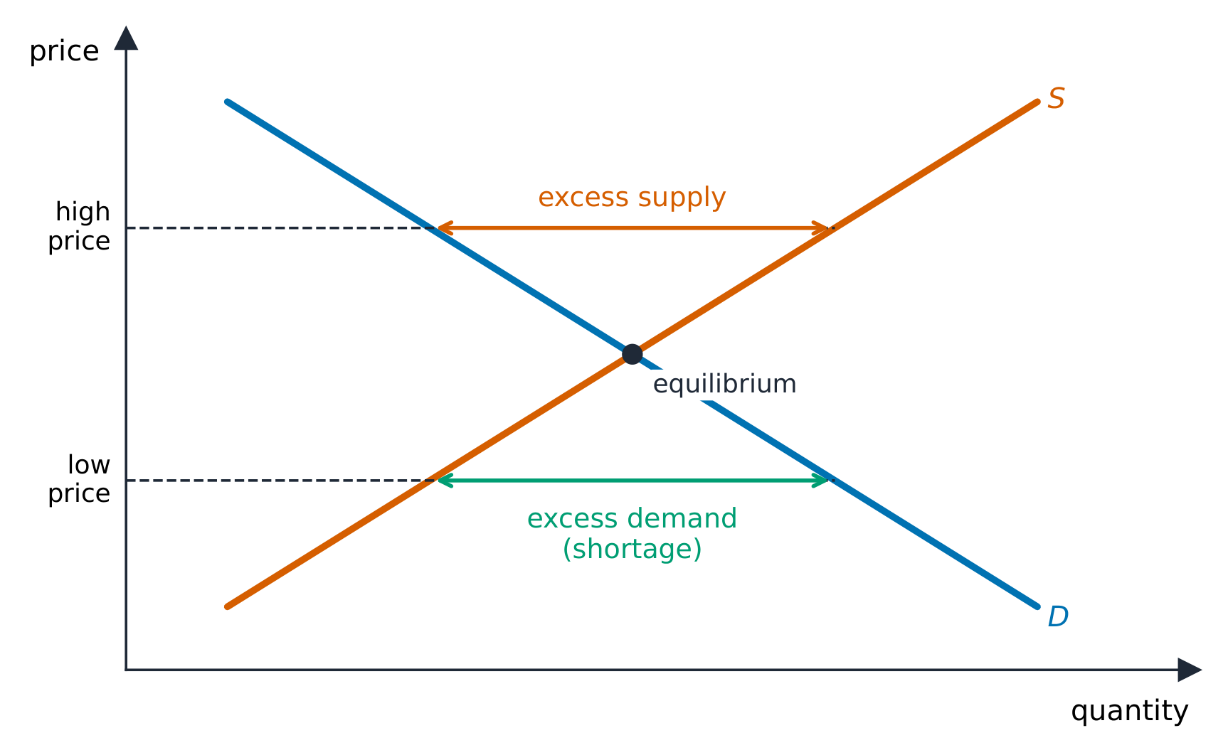
Away from equilibrium the market self-corrects: above the equilibrium price there is a surplus 过剩 (excess supply) that pushes price down; below it a shortage 短缺 (excess demand) that pushes price up.
When a determinant shifts a curve, the equilibrium moves predictably. A single shift gives a definite result for both price and quantity. When both curves shift, one of price or quantity is indeterminate (depends on the relative sizes of the shifts) – a favorite exam trap. Work these out by drawing the shifts.
Vocabulary
Train
| English |
|---|
| surplus/ˈsɜːpləs/ |
| shortage/ˈʃɔːtɪdʒ/ |
2.8
The Effects of Government Intervention in Markets
Syllabus
| Enduring Understanding | Learning Objective | Essential Knowledge |
|---|---|---|
POL-1 | POL-1.A |
|
Source: College Board AP Course and Exam Description
Start with an initially efficient competitive market. Binding interventions can reduce total surplus; a policy correcting a market failure can instead improve social welfare (Unit 6).
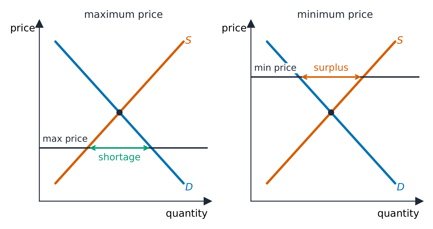
- A price ceiling 价格上限 (a legal maximum, like rent control) below equilibrium causes a persistent shortage.
- A price floor 价格下限 (a legal minimum, like a minimum wage) above equilibrium causes a persistent surplus.
- A per-unit excise tax 消费税 on sellers shifts supply up by the tax; the burden (tax incidence 税收归宿) falls more heavily on whichever side is more inelastic.
- A per-unit producer subsidy shifts supply down, raising quantity.
Deadweight loss 无谓损失 is lost total surplus. In this initially efficient model, a tax prevents some beneficial trades; a subsidy can encourage units whose cost exceeds their benefit. A nonbinding price control has no effect on the market outcome.
Worked controls. Use $P_D=20-Q$ and $P_S=2+Q$, so the original equilibrium is $P^*=\$11$, $Q^*=9$. At a ceiling of $\$8$:
$$Q_d=20-P=20-8=12,\qquad Q_s=P-2=8-2=6.$$
$$\text{Shortage}=Q_d-Q_s=12-6=6\text{ units}.$$
At most six units trade without other supply. At a floor of $\$14$, $Q_d=6$ and $Q_s=12$, so the surplus is six units; without government purchases, buyers take at most six units.
Worked tax. A $\$4$ tax per unit creates a wedge between the buyer price $P_b$ and seller receipt $P_s$:
$$P_b=P_s+t,\qquad20-Q=2+Q+4.$$
$$Q_t=7,\qquad P_b=\$13,\qquad P_s=\$9.$$
Tax incidence. Buyers pay $\$2$ more and sellers receive $\$2$ less than before; the burden is equal for these symmetric schedules. Generally, the relatively more inelastic side bears more.
$$\text{Tax revenue}=tQ_t=4(7)=\$28.$$
$$DWL=\tfrac12t(Q^*-Q_t)=\tfrac12(4)(9-7)=\$4.$$
Government revenue is a transfer, not the deadweight loss.
Exam skill: on a graph, be able to shade consumer surplus, producer surplus, government revenue from a tax, and deadweight loss, and say who bears the tax and why.
Explore
Add a tax or price control
A price ceiling below equilibrium causes shortages; a tax drives a wedge between what buyers pay and sellers get, shrinking the quantity traded.
Vocabulary
Train
| English |
|---|
| price ceiling/praɪs ˈsiːlɪŋ/ |
| price floor/praɪs flɔː/ |
| excise tax/ekˈsaɪz tæks/ |
| tax incidence/tæks ˈɪnsɪdəns/ |
| deadweight loss/ˈdedweɪt lɒs/ |
2.9
International Trade and Public Policy
Syllabus
| Enduring Understanding | Learning Objective | Essential Knowledge |
|---|---|---|
POL-1 | POL-1.B |
|
Source: College Board AP Course and Exam Description
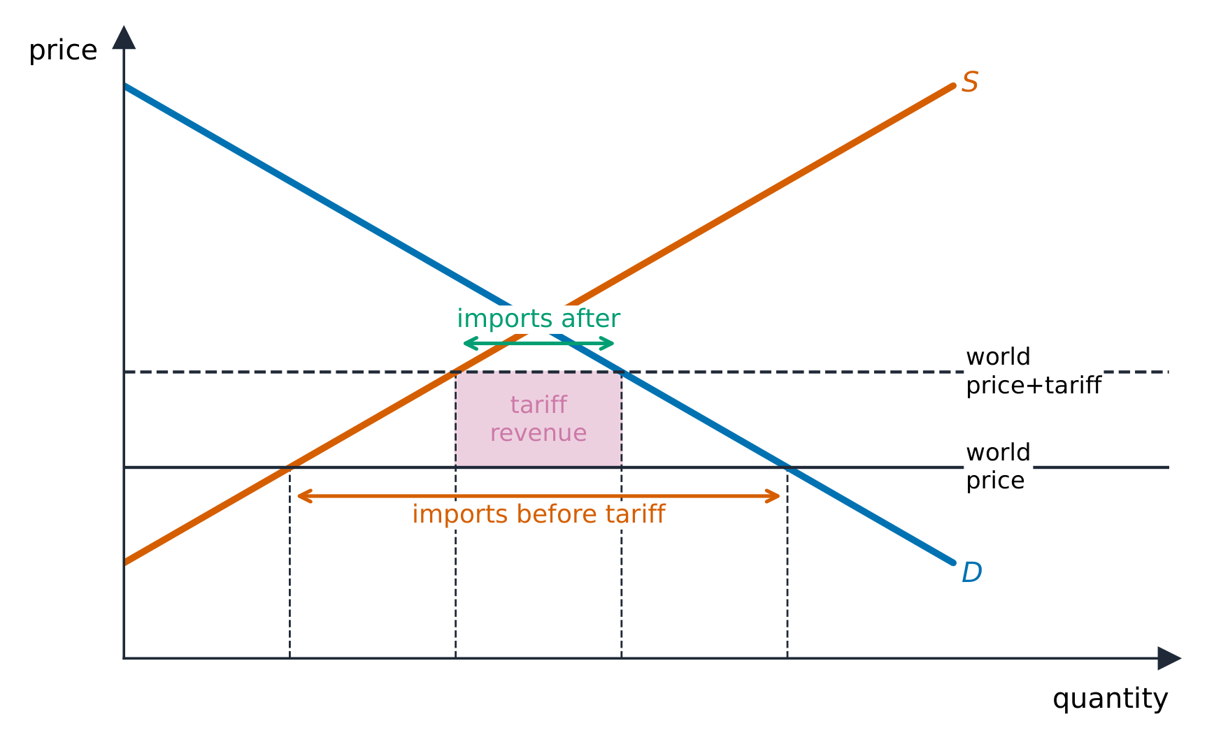
In the competitive small-country model, the country takes the world price 世界价格 as given. Assume no external costs or benefits. Compare it with the domestic price before trade:
- If the world price is below the domestic price, the country imports 进口 – consumers gain more than producers lose, so total surplus rises.
- If the world price is above the domestic price, the country exports 出口 – producers gain more than consumers lose.
A binding tariff 关税 (import tax) or quota 配额 (import limit) raises domestic price and reduces total surplus in this model. Domestic curves do not shift.
Worked imports and tariff. Keep $P_D=20-Q$ and $P_S=2+Q$. The world price is $\$6$, below the $\$11$ no-trade equilibrium.
$$Q_d=20-P_w=14,\quad Q_s=P_w-2=4,\quad M=Q_d-Q_s=10.$$
A $\$2$ tariff raises the domestic price to $\$8$; imports continue because this is below $\$11$.
$$Q_{d,t}=20-8=12,\quad Q_{s,t}=8-2=6,\quad M_t=12-6=6.$$
$$\text{Tariff revenue}=tM_t=2(6)=\$12.$$
The production and consumption distortions each lose a triangle of surplus:
$$DWL=\tfrac12t[(Q_{s,t}-Q_s)+(Q_d-Q_{d,t})]=\tfrac12(2)[(6-4)+(14-12)]=\$4.$$
These are conditional model results, not a claim that every real-world trade policy has the same welfare effect.
Vocabulary
Train
| English |
|---|
| world price/wɜːld praɪs/ |
| imports/ɪmˈpɔːts/ |
| exports/ˈekspɔːts/ |
| tariff/ˈtærɪf/ |
| quota/ˈkwəʊtə/ |
2.9
Exam tips
- Separate a movement along a curve (own price) from a shift (a determinant); a single shift gives a definite result, a double shift leaves one variable indeterminate.
- Compute elasticity $E_d=|\%\Delta Q \div \%\Delta P|$; elastic ($>1$) means a price cut raises total revenue, inelastic ($<1$) lowers it.
- Read the sign of cross-price elasticity (substitutes $+$, complements $-$) and income elasticity (normal $+$, inferior $-$).
- Shade consumer/producer surplus and the deadweight loss from a tax or price control; incidence falls on the more inelastic side.
- A price ceiling below equilibrium causes a shortage; a price floor above causes a surplus.
Interactive lessons on this topic
Work through it step by step, with instant-check exercises.