| Enduring Understanding | Learning Objective | Essential Knowledge |
|---|---|---|
MOD-2 | MOD-2.A |
|
National Income and Price Determination
AP Macroeconomics · Topic 3
 8:50
8:50
National Income and Price Determination
A government spends ten billion dollars on new railways. How much does the country's output rise? Not ten billion. It can rise by fifty billion. Money spent by…
English narration · English + 中文 subtitles burned in
3.1
Aggregate Demand

Syllabus
Source: College Board AP Course and Exam Description
Aggregate demand (AD) 总需求 shows the total quantity of real output ($C+I+G+X_n$) buyers want at each price level 价格水平. It slopes downward for three reasons special to the whole economy:
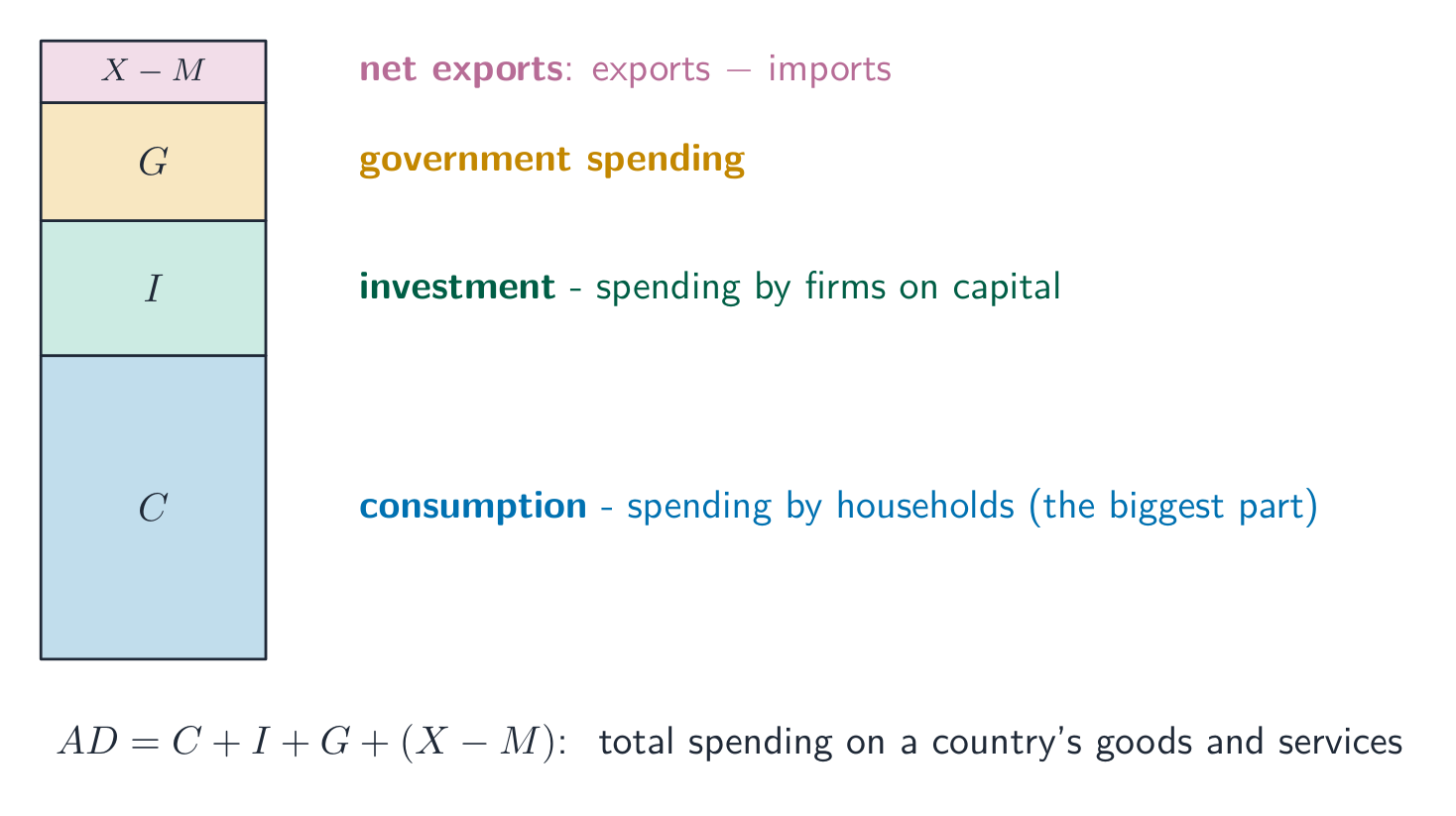
- the wealth effect 财富效应 (a higher price level shrinks the real value of money, so people buy less),
- the interest-rate effect 利率效应 (a higher price level raises money demand and interest rates, cutting investment),
- the net-export effect (a higher domestic price level makes exports dearer and imports cheaper).
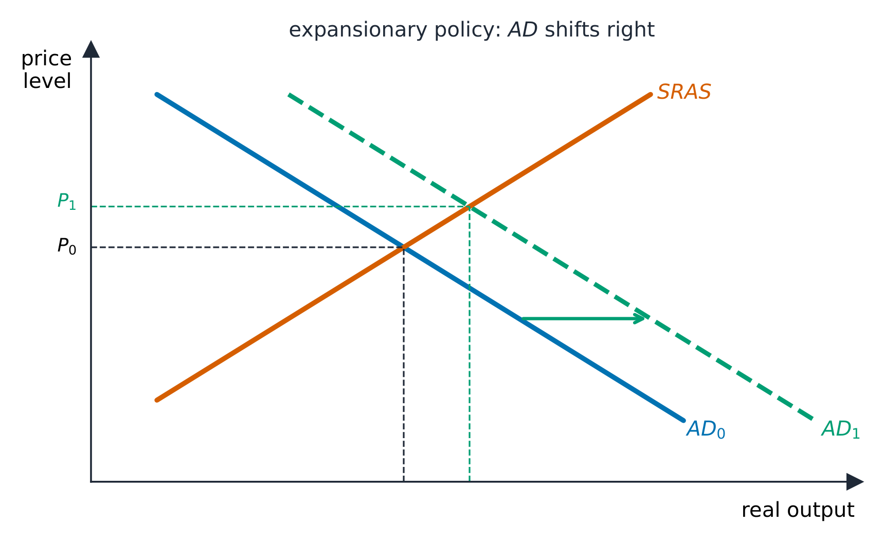
A change in the price level is a movement along AD. AD shifts when any component of $C+I+G+X_n$ changes for another reason – consumer confidence, business expectations, government spending, taxes, or foreign incomes.
Vocabulary
Train
| English |
|---|
| Aggregate demand (AD)/ˈæɡrɪɡeɪt dɪˈmænd/ |
| price level/praɪs ˈlevl/ |
| wealth effect/welθ ɪˈfekt/ |
| interest-rate effect/ˈɪntrest reɪt ɪˈfekt/ |
3.2
The Spending and Tax Multipliers
Syllabus
| Enduring Understanding | Learning Objective | Essential Knowledge |
|---|---|---|
MOD-2 | MOD-2.B |
|
Source: College Board AP Course and Exam Description
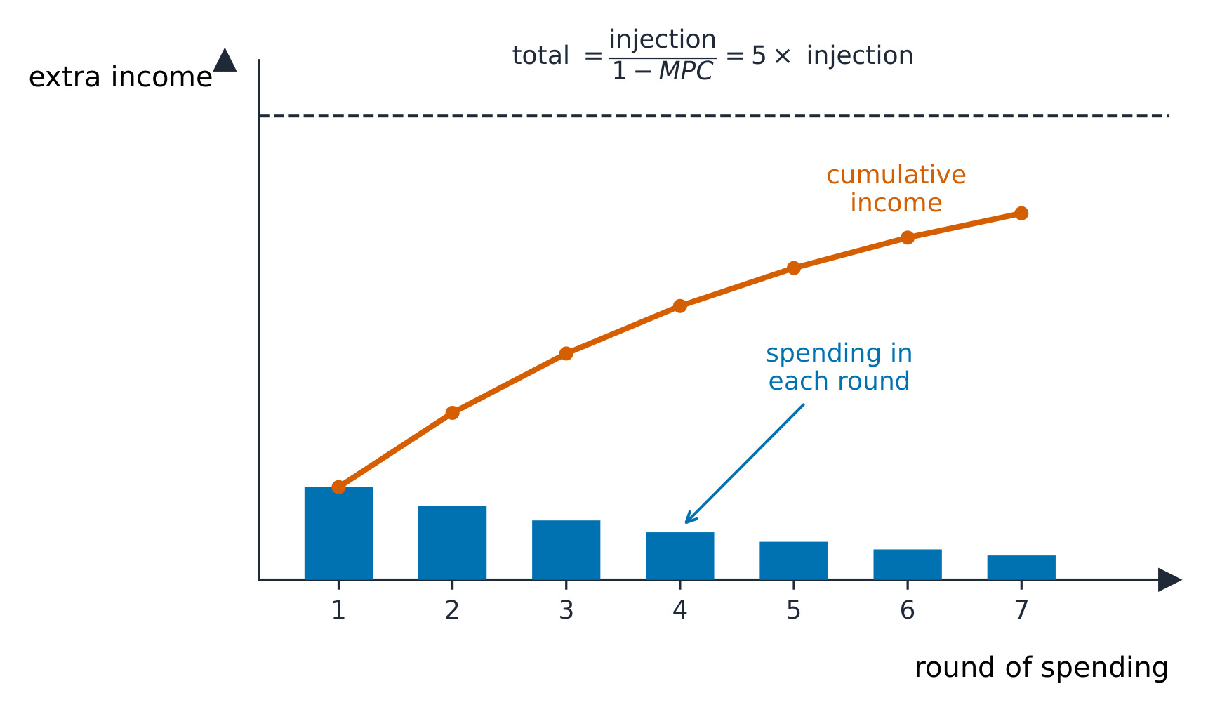
A change in spending sets off further rounds of spending, so the final change in GDP is larger than the initial change – the multiplier effect 乘数效应. It depends on the marginal propensity to consume 边际消费倾向 (MPC), the fraction of extra income that is spent (the rest is the marginal propensity to save 边际储蓄倾向, MPS, with $MPC+MPS=1$):
$$\text{spending multiplier}=\frac{1}{1-MPC}=\frac{1}{MPS}.$$
A tax cut works through the multiplier too, but more weakly, because part of the tax cut is saved:
$$\text{tax multiplier}=-\frac{MPC}{1-MPC}=-\frac{MPC}{MPS}.$$
The tax multiplier is smaller in size and negative (a tax cut raises GDP; a tax rise lowers it). Total change in GDP $=$ (multiplier) $\times$ (initial change).
Worked example. If $MPC=0.8$, the spending multiplier is $\dfrac{1}{1-0.8}=5$, so a $\$10$ billion rise in government spending lifts real GDP by $5\times\$10=\$50$ billion. The tax multiplier is $-\dfrac{0.8}{0.2}=-4$, so a $\$10$ billion tax cut raises GDP by only $\$40$ billion – weaker, because part of the tax cut is saved.
Exam skill: compute both multipliers from the MPC and find the resulting change in real GDP – an almost-guaranteed calculation.
Explore
See the spending multiplier ripple out
A dollar of new spending becomes someone's income, part of which they spend again — so the total effect is a multiple of the first injection, set by the marginal propensity to consume (MPC).
Vocabulary
Train
| English |
|---|
| multiplier effect/ˌmʌltɪˈplaɪə ɪˈfekt/ |
| marginal propensity to consume/ˈmɑːdʒɪnl prəˈpensɪti tə kənˈsjuːm/ |
| marginal propensity to save/ˈmɑːdʒɪnl prəˈpensɪti tə seɪv/ |
3.3
Short-Run Aggregate Supply

Syllabus
| Enduring Understanding | Learning Objective | Essential Knowledge |
|---|---|---|
MOD-2 | MOD-2.C |
|
MOD-2.D |
|
Source: College Board AP Course and Exam Description
Short-run aggregate supply (SRAS) 短期总供给 slopes upward: in the short run some input prices (especially nominal wages 名义工资) are sticky 粘性, so a higher output price level widens profit margins and firms produce more. SRAS shifts with input prices, productivity, taxes/subsidies on producers, and supply shocks (e.g. an oil-price change). A rise in input costs shifts SRAS left.
Vocabulary
Train
| English |
|---|
| Short-run aggregate supply (SRAS)/ʃɔːt rʌn ˈæɡrɪɡeɪt səˈplaɪ/ |
| nominal wages/ˈnɒmɪnl ˈweɪdʒɪz/ |
| sticky/ˈstɪki/ |
3.4
Long-Run Aggregate Supply
Syllabus
| Enduring Understanding | Learning Objective | Essential Knowledge |
|---|---|---|
MOD-2 | MOD-2.E |
|
MOD-2.F |
|
Source: College Board AP Course and Exam Description
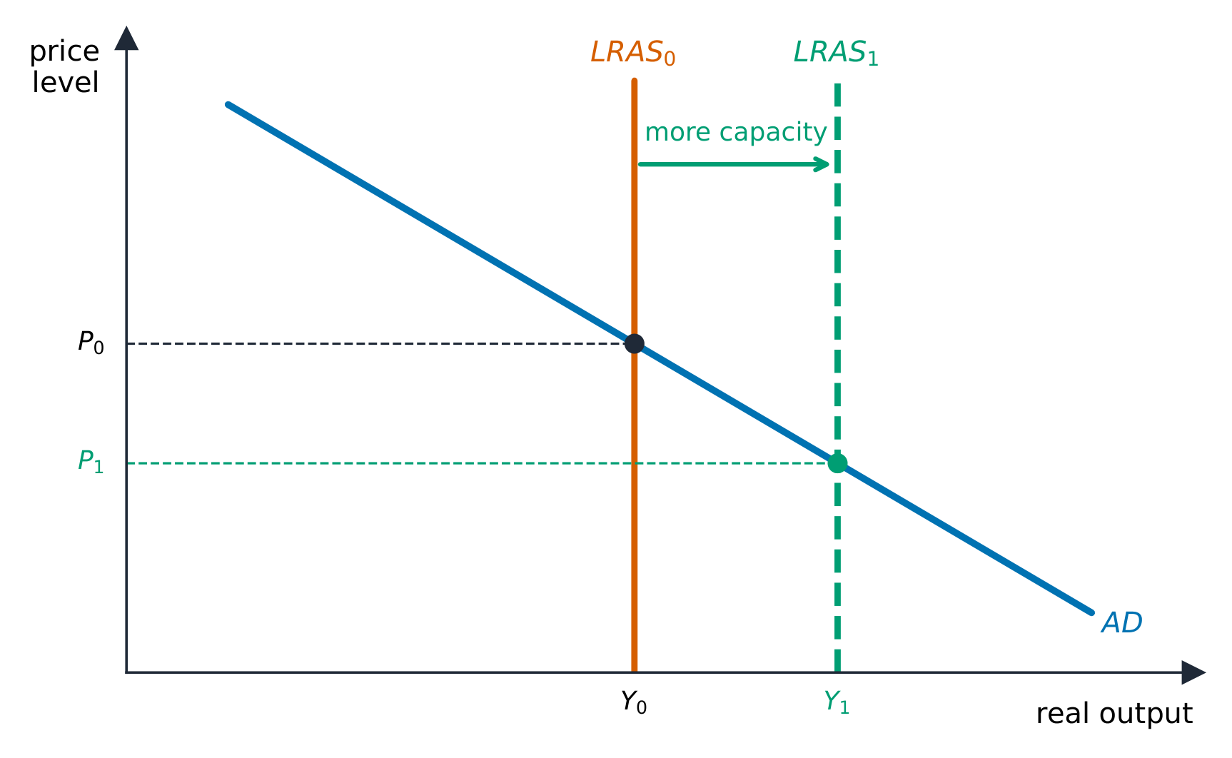
Long-run aggregate supply (LRAS) 长期总供给 is vertical at the economy's full-employment (potential) output 潜在产出 $Y_f$. In the long run all prices and wages are fully flexible (only in the short run are some input prices fixed), so output depends only on real factors – resources, technology, institutions – not the price level. LRAS shifts only with economic growth (more or better resources). LRAS corresponds to the production possibilities curve (PPC) 生产可能性曲线: both mark the economy's maximum sustainable capacity, so an outward LRAS shift and an outward PPC shift are the same event drawn two ways. The vertical LRAS is why, in the long run, demand policy changes prices, not output.
Vocabulary
Train
| English |
|---|
| Long-run aggregate supply (LRAS)/lɒŋ rʌn ˈæɡrɪɡeɪt səˈplaɪ/ |
| full-employment (potential) output/fʊl emˈplɔɪmənt ˈaʊtpʊt/ |
| production possibilities curve (PPC)/prəˈdʌkʃn ˌpɒsəˈbɪlɪtiz kɜːv/ |
3.5
Equilibrium in the AD-AS Model
Syllabus
| Enduring Understanding | Learning Objective | Essential Knowledge |
|---|---|---|
MOD-2 | MOD-2.G |
|
Source: College Board AP Course and Exam Description
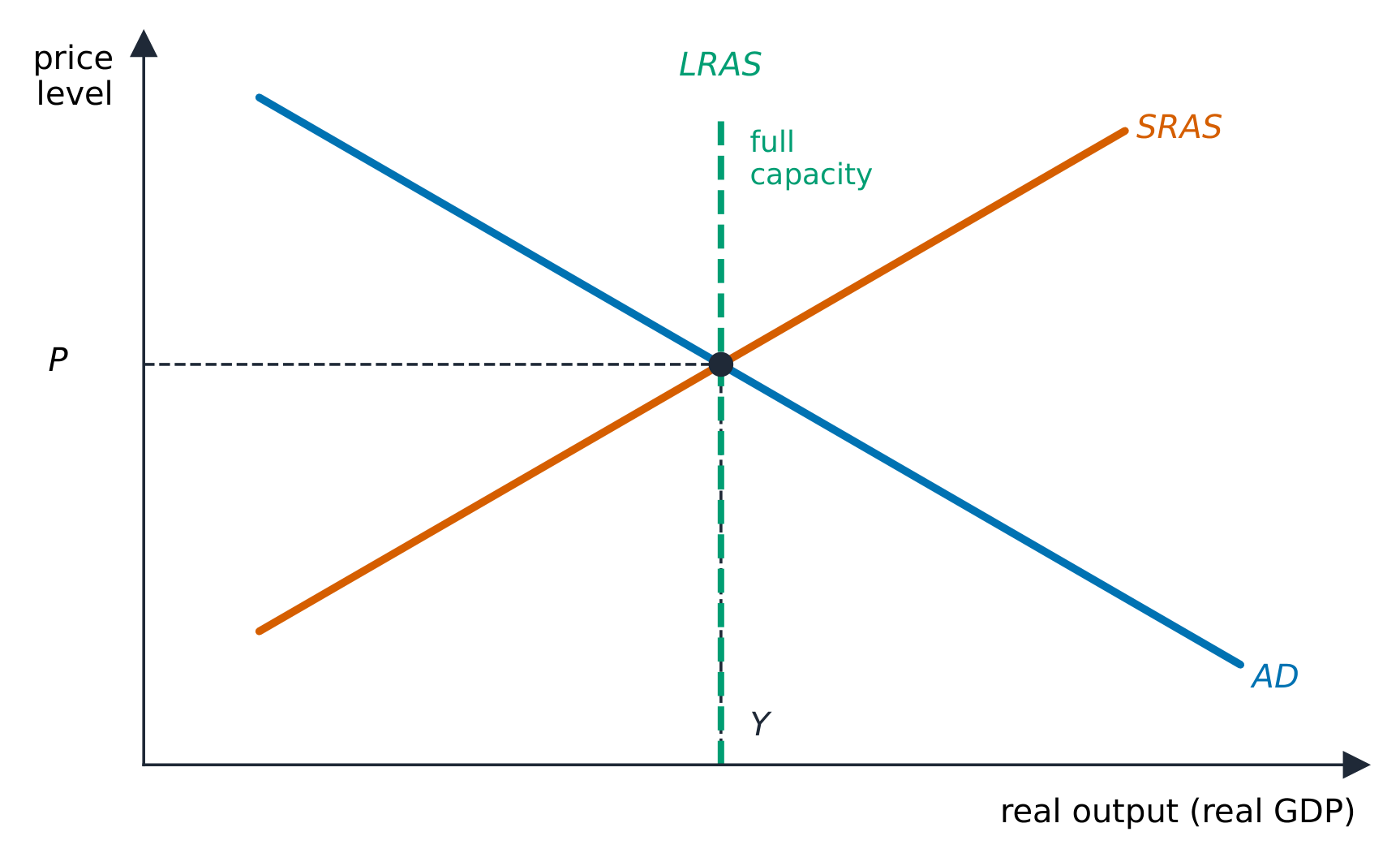
The economy settles where AD meets SRAS, fixing the equilibrium price level and real GDP. Comparing that output to $Y_f$ (the LRAS line) gives the economy's state:
- output $
- output $>Y_f$: an inflationary gap 通胀缺口 (overheating),
- output $=Y_f$: long-run equilibrium.
Explore
Find equilibrium in the AD-AS model
Aggregate demand and aggregate supply cross at the economy's price level and real GDP. A demand or supply shock shifts a curve and moves the whole economy's output and prices.
Vocabulary
Train
| English |
|---|
| recessionary gap/rɪˈseʃənəri ɡæp/ |
| inflationary gap/ɪnˈfleɪʃənəri ɡæp/ |
3.6
Short-Run Changes: Demand and Supply Shocks
Syllabus
| Enduring Understanding | Learning Objective | Essential Knowledge |
|---|---|---|
MOD-2 | MOD-2.H |
|
Source: College Board AP Course and Exam Description
- A demand shock shifts AD: a positive one (more spending) raises both price level and output (and lowers unemployment); a negative one lowers both.
- A supply shock shifts SRAS: a negative one (higher input costs) raises the price level and lowers output at once – stagflation 滞胀 – the hardest case for policymakers, because fixing one worsens the other.
Vocabulary
Train
| English |
|---|
| stagflation/stæɡˈfleɪʃn/ |
3.7
Long-Run Self-Adjustment
Syllabus
| Enduring Understanding | Learning Objective | Essential Knowledge |
|---|---|---|
MOD-2 | MOD-2.I |
|
Source: College Board AP Course and Exam Description
Left alone, the economy self-corrects through flexible wages:
- In a recessionary gap, high unemployment eventually pushes nominal wages down, shifting SRAS right until output returns to $Y_f$ at a lower price level.
- In an inflationary gap, labor shortages push wages up, shifting SRAS left back to $Y_f$ at a higher price level.
The debate over how fast this happens is the case for (or against) active policy: self-adjustment is slow and painful, which is the argument for intervening.
3.8
Fiscal Policy
Syllabus
| Enduring Understanding | Learning Objective | Essential Knowledge |
|---|---|---|
POL-1 | POL-1.A |
|
POL-1.B |
|
Source: College Board AP Course and Exam Description
Fiscal policy 财政政策 is the government's use of spending and taxes to shift AD:
- Expansionary 扩张性 (more spending or lower taxes) shifts AD right to close a recessionary gap.
- Contractionary 紧缩性 (less spending or higher taxes) shifts AD left to close an inflationary gap.
Size the policy with the multipliers: to close a gap of a given size, the required change in spending is (gap) $\div$ (spending multiplier). Limits include time lags, crowding out (below), and political difficulty.
Worked example. An economy has a $\$100$ billion recessionary gap and $MPC=0.75$ (spending multiplier $=\dfrac{1}{0.25}=4$). To close it, the government must raise spending by $\dfrac{\$100\text{ billion}}{4}=\$25$ billion. Using a tax cut instead (tax multiplier $-3$) would require a larger $\dfrac{100}{3}\approx\$33$ billion cut.
Exam skill: you must draw the correctly labeled AD-AS graph, identify the gap, prescribe the right fiscal action and its direction, and often calculate the exact spending or tax change needed.
Vocabulary
Train
| English |
|---|
| Fiscal policy/ˈfɪskl ˈpɒlɪsi/ |
| Expansionary/ekˈspænʃənəri/ |
| Contractionary/kənˈtrækʃənəri/ |
3.9
Automatic Stabilizers
Syllabus
| Enduring Understanding | Learning Objective | Essential Knowledge |
|---|---|---|
POL-1 | POL-1.C |
|
Source: College Board AP Course and Exam Description
Automatic stabilizers 自动稳定器 are features that dampen the cycle without new legislation. In a downturn, progressive taxes collect less and transfer payments (unemployment benefits, welfare) rise automatically – cushioning incomes and spending; in a boom they do the reverse. They soften the cycle and act instantly, avoiding the lags of discretionary 相机抉择 policy.
Vocabulary
Train
| English |
|---|
| Automatic stabilizers/ˌɔːtəˈmætɪk ˈsteɪbəlaɪzəz/ |
| discretionary/dɪˈskreʃənəri/ |
3.9
Exam tips
- Aggregate demand slopes down for the wealth, interest-rate, and net-export effects; it shifts when $C$, $I$, $G$, or $X_n$ changes.
- Compute the spending multiplier $\tfrac{1}{1-MPC}$ and the smaller, negative tax multiplier $-\tfrac{MPC}{1-MPC}$.
- Draw a correctly labeled AD–AS graph, identify a recessionary or inflationary gap, and prescribe the right fiscal action.
- Short-run AS slopes up (sticky wages); long-run AS is vertical at full-employment output.
- Size a policy with the multipliers: required spending = gap ÷ spending multiplier.
Interactive lessons on this topic
Work through it step by step, with instant-check exercises.