| Enduring Understanding | Learning Objective | Essential Knowledge |
|---|---|---|
FUN-7 | FUN-7.A |
|
Differential Equations
AP Calculus BC · Topic 7
 8:26
8:26
Modeling with Differential Equations
Normally you are handed a function and asked for its slope. A differential equation turns that around. You are handed a rule for the slope at every point, and…
English narration · English + 中文 subtitles burned in
7.1
Modeling Situations with Differential Equations
Syllabus
Source: College Board AP Course and Exam Description
A differential equation 微分方程 relates a function to its derivatives. Many real situations are described by a rate: "the population grows at a rate proportional to its size" becomes $\dfrac{dP}{dt}=kP$. Setting up the equation from a verbal description – identifying what changes and what it is proportional to – is the first skill.
Vocabulary
Train
| English |
|---|
| differential equation/ˌdɪfəˈrenʃl ɪˈkweɪʒn/ |
7.2
Verifying Solutions for Differential Equations
Syllabus
| Enduring Understanding | Learning Objective | Essential Knowledge |
|---|---|---|
FUN-7 | FUN-7.B |
|
Source: College Board AP Course and Exam Description
A solution is a function that satisfies the equation. To verify a proposed solution, differentiate it and substitute into the equation, checking that both sides agree. A general solution contains a constant $C$; a particular solution fixes $C$ from a condition.
7.3
Sketching Slope Fields
Syllabus
| Enduring Understanding | Learning Objective | Essential Knowledge |
|---|---|---|
FUN-7 | FUN-7.C |
|
Source: College Board AP Course and Exam Description
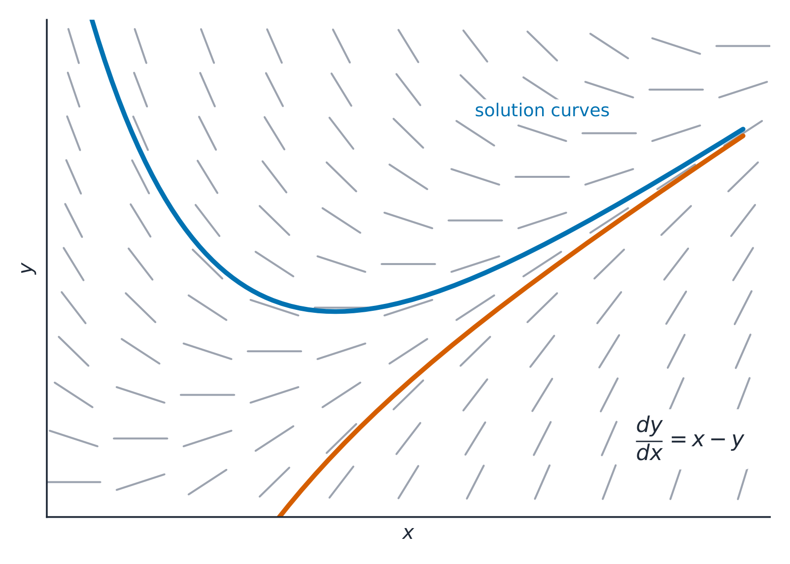
A slope field 斜率场 draws a short line segment at many points, each with the slope $\dfrac{dy}{dx}$ the equation gives there. It pictures the family of solution curves without solving. To sketch one, evaluate the right-hand side at each grid point and draw a segment of that slope.
Explore
Read a differential equation as a slope field
A slope field draws the slope $dy/dx$ at each point. A solution curve threads through, always tangent to the little segments — you can sketch it by following the flow.
Vocabulary
Train
| English |
|---|
| slope field/sləʊp fiːld/ |
7.4
Reasoning Using Slope Fields
Syllabus
| Enduring Understanding | Learning Objective | Essential Knowledge |
|---|---|---|
FUN-7 | FUN-7.C |
|
Source: College Board AP Course and Exam Description
A solution curve follows the segments like a boat following a current. From a slope field you can sketch the particular solution through a given point, describe long-run behavior, and locate where solutions level off (slopes near zero) – reasoning about solutions purely from the picture.
7.5
Approximating Solutions Using Euler's Method
Syllabus
| Enduring Understanding | Learning Objective | Essential Knowledge |
|---|---|---|
FUN-7 | FUN-7.C |
|
Source: College Board AP Course and Exam Description
Euler's method 欧拉方法 approximates a solution numerically by stepping along the slope field. Starting from a known point, take a small step $\Delta x$ and update:
$$y_{\text{new}}=y_{\text{old}}+\frac{dy}{dx}\cdot\Delta x.$$
Repeat for each step. Smaller steps give a better approximation. (This is a BC-only technique.)
Exam skill: be able to carry out two or three Euler steps by hand from a table, and know that Euler's method under- or over-estimates depending on the solution's concavity.
Worked example. Approximate $y(1)$ for $\dfrac{dy}{dx}=x+y$, $y(0)=1$, with step $\Delta x=0.5$. Step 1: slope at $(0,1)$ is $0+1=1$, so $y(0.5)\approx 1+1(0.5)=1.5$. Step 2: slope at $(0.5,1.5)$ is $0.5+1.5=2$, so $y(1)\approx 1.5+2(0.5)=2.5$.
Vocabulary
Train
| English |
|---|
| Euler's method/ˈɔɪləz ˈmeθəd/ |
7.6
Finding General Solutions Using Separation of Variables
Syllabus
| Enduring Understanding | Learning Objective | Essential Knowledge |
|---|---|---|
FUN-7 | FUN-7.D |
|
Source: College Board AP Course and Exam Description
A separable 可分离 differential equation can be written with all the $y$'s on one side and all the $x$'s on the other, then integrated:
$$\frac{dy}{dx}=g(x)h(y)\ \Rightarrow\ \int\frac{dy}{h(y)}=\int g(x)\,dx.$$
This produces the general solution (with a $+C$), the main analytic method for solving differential equations in this course.
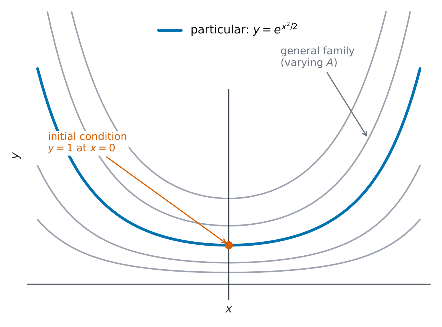
Worked example. Solve $\dfrac{dy}{dx}=xy$ with $y(0)=2$. Separating, $\int\frac{dy}{y}=\int x\,dx$ gives $\ln|y|=\frac{x^2}{2}+C$, so $y=Ae^{x^2/2}$. The condition $y(0)=2$ gives $A=2$, so $y=2e^{x^2/2}$.
Vocabulary
Train
| English |
|---|
| separable/ˈsepərəbl/ |
7.7
Finding Particular Solutions Using Initial Conditions
Syllabus
| Enduring Understanding | Learning Objective | Essential Knowledge |
|---|---|---|
FUN-7 | FUN-7.E |
|
Source: College Board AP Course and Exam Description
An initial condition 初始条件 (a known point, e.g. $y(0)=5$) pins down the constant $C$. Solve for the general solution, substitute the condition to find $C$, then write the particular solution. Watch the domain – a particular solution is valid only on the interval containing the initial point.
Vocabulary
Train
| English |
|---|
| initial condition/ɪˈnɪʃl kənˈdɪʃn/ |
7.8
Exponential Models with Differential Equations

Syllabus
| Enduring Understanding | Learning Objective | Essential Knowledge |
|---|---|---|
FUN-7 | FUN-7.F |
|
FUN-7.G |
|
Source: College Board AP Course and Exam Description
The equation $\dfrac{dy}{dt}=ky$ says the rate of change is proportional to the amount – giving exponential growth or decay 指数增长. Separating variables yields
$$y=y_0 e^{kt},$$
with $k>0$ for growth and $k<0$ for decay. This models unrestricted population growth, radioactive decay, and continuously compounded interest.
Explore
An exponential growth/decay model
y = a·e^(bx) + c
The equation $dy/dt=ky$ has exponential solutions: quantity changes at a rate proportional to itself, giving unbounded growth ($k>0$) or decay to zero ($k<0$).
Vocabulary
Train
| English |
|---|
| exponential growth or decay/ˌekspəˈnenʃl ɡrəʊθ ɔː dɪˈkeɪ/ |
7.9
Logistic Models with Differential Equations
Syllabus
| Enduring Understanding | Learning Objective | Essential Knowledge |
|---|---|---|
FUN-7 | FUN-7.H |
|
Source: College Board AP Course and Exam Description
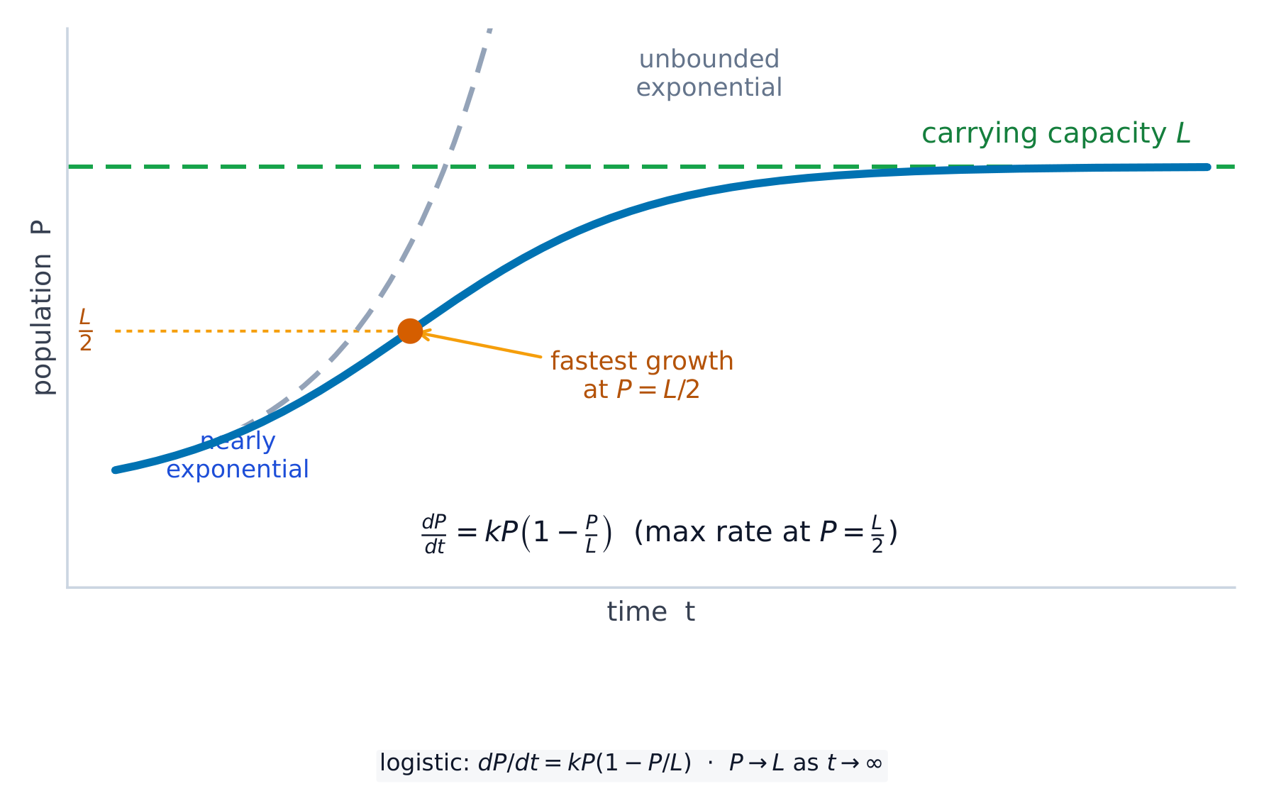
Real growth is limited by resources, so the logistic model 逻辑斯蒂模型 adds a carrying capacity 环境容纳量 $L$:
$$\frac{dP}{dt}=kP\!\left(1-\frac{P}{L}\right).$$
Growth is nearly exponential when $P$ is small, slows as $P$ approaches $L$, and stops at $P=L$. Key BC facts: the population levels off at $L$ ($\lim_{t\to\infty}P=L$), and it grows fastest when $P=\tfrac{L}{2}$ (the inflection point of the S-shaped curve). You are expected to read $L$ and the fastest-growth value directly from the equation.
Worked example. For $\dfrac{dP}{dt}=0.05\,P\!\left(1-\dfrac{P}{2000}\right)$, the carrying capacity is $L=2000$ (the population levels off there), and growth is fastest when $P=\dfrac{L}{2}=1000$ – both read straight off the equation, no solving needed.
Vocabulary
Train
| English |
|---|
| logistic model/ləˈdʒɪstɪk ˈmɒdl/ |
| carrying capacity/ˈkæriɪŋ kəˈpæsɪti/ |
7.9
Exam tips
- Solve a separable equation by getting all $y$ on one side and all $x$ on the other, then integrating both sides (add $+C$ once).
- Use the initial condition to find $C$ (a particular solution).
- Sketch or read a slope field: the little segments show $\tfrac{dy}{dx}$ at each point, and a solution curve follows them.
- Recognise exponential models $\tfrac{dy}{dt}=ky\Rightarrow y=Ce^{kt}$ (growth/decay).
- A differential equation gives the slope — you must integrate to recover the function.
Interactive lessons on this topic
Work through it step by step, with instant-check exercises.
- Modeling Situations with Differential Equations
- Verifying Solutions for Differential Equations
- Sketching Slope Fields
- Reasoning Using Slope Fields
- Approximating Solutions Using Euler's Method
- Finding General Solutions Using Separation of Variables
- Finding Particular Solutions Using Initial Conditions and Separation of Variables
- Exponential Models with Differential Equations
- Logistic Models with Differential Equations