Uncertainty, gradients and model testing
Introduit| English | Sens |
|---|---|
| systematic error/ˌsɪstəˈmætɪk ˈerə/ | erreur systématique |
| uncertainty/ʌnˈsɜːtənti/ | incertitude |
What would explain this observation?
- A line passing near every data point is useful, but its gradient can still be uncertain. A graph is evidence for a model within the measurement range.
Build the model
- Random variation makes repeated readings differ.
- Systematic error 系统误差 shifts results consistently.
- Absolute uncertainty 不确定度 has the measured unit; relative or percentage uncertainty compares uncertainty with the measured value.
- uncertainty: A quantified limitation on a measured result.
- systematic error: A consistent measurement bias.

Which is most likely a systematic error?
Difficulté 1/5 · 100 pièces + un petit bonus lors de la première réussite aujourd'hui
A fixed 0.20 g balance zero offset is a systematic error. Independent repeats reduce random uncertainty in the mean, not scatter in individual readings or a shared offset. Reaction timing can have both random and systematic contributions.
Match each technical term to its precise meaning.
Difficulté 2/5 · 140 pièces + un petit bonus lors de la première réussite aujourd'hui
Use the definitions to distinguish related quantities and processes.
Choose evidence that can test it
- For a product or quotient, adding fractional uncertainties is a common maximum-uncertainty approximation.
- For a difference, add absolute uncertainties.
- A nonzero intercept can reveal an offset or an incomplete model.
In the lab: Show units on axes and choose a sensible scale. Plot uncertainty bars where justified, draw a best-fit line rather than joining every point, and estimate steepest and shallowest plausible gradients when the course method calls for them.
Which two habits make the investigation or model in this case more defensible?
Difficulté 2/5 · 140 pièces + un petit bonus lors de la première réussite aujourd'hui
Stating the conditions and assumptions lets others repeat the work exactly, and recording the supporting evidence lets them check the conclusion. Hiding disagreeing results removes the evidence that could challenge a wrong conclusion, and one measurement can never establish a wider claim.
Work from known quantities
- Known: length = 50.0 mm with uncertainty 1.0 mm.
- Percentage uncertainty = absolute uncertainty/value ×100 = 1.0/50.0×100 = 2.0%.
- For a quotient of two independently measured quantities with maximum percentage uncertainties 2% and 3%, the summed maximum estimate is 5%.
Your turn: A 40 cm reading has an absolute uncertainty of 1 cm. Find percentage uncertainty.
Measurement ranges and the quotient estimate
50 ± 1 mm has a 2% uncertainty. Compare it with a 100 ± 3 mm reading: the summed quotient estimate is 5%, while exact endpoint calculations reveal a slightly asymmetric range.
A 40 cm reading has an absolute uncertainty of 1 cm. Find percentage uncertainty.
Difficulté 2/5 · 140 pièces + un petit bonus lors de la première réussite aujourd'hui
The result is 2.5 %. Known: reading 40 cm; absolute uncertainty 1 cm. Use percentage uncertainty = absolute uncertainty / value x 100. Percentage uncertainty = 1/40 x 100 = 2.5%. Smaller measured values carry larger percentage uncertainties for the same absolute uncertainty.
Check the conclusion and its limits
- Repeating readings reduces random uncertainty in a mean but does not automatically remove a zero error.
- Do not quote more decimal places than your measurement can support.
Not true: Repeating a measurement always removes a calibration offset. Independent repeats and averaging can reduce random uncertainty of the mean, while a calibration offset can remain. Check calibration and apply a justified correction where appropriate.
- Random variation makes repeated readings differ.
- For a product or quotient, adding fractional uncertainties is a common maximum-uncertainty approximation.
- Watch for: repeating readings reduces random uncertainty in a mean but does not automatically remove a zero error.
Repeating a measurement always removes a calibration offset.
Difficulté 1/5 · 100 pièces + un petit bonus lors de la première réussite aujourd'hui
Independent repeats and averaging can reduce random uncertainty of the mean, while a calibration offset can remain. Check calibration and apply a justified correction where appropriate.
A quantified limitation on a measured result: write the technical term.
Difficulté 1/5 · 100 pièces + un petit bonus lors de la première réussite aujourd'hui
uncertainty means A quantified limitation on a measured result.
Write from the data: find the percentage uncertainty
- An 80 cm reading has an absolute uncertainty of 4 cm.
- Find the percentage uncertainty. Repeating the reading does not remove a calibration offset.
An 80 cm reading has an absolute uncertainty of 4 cm. What is the percentage uncertainty, and why does repeating the measurement not remove a calibration offset?
Fractional uncertainty = ΔL/|L| = 4/80 = 0.05. Multiplying by 100 gives 5%. Independent repeats can reduce random uncertainty in the mean; a shared calibration offset shifts all readings together and remains unless corrected.
A reading is 80 cm with absolute uncertainty 4 cm. What is the percentage uncertainty?
Difficulté 1/5 · 100 pièces + un petit bonus lors de la première réussite aujourd'hui
4 divided by 80 is 0.05, so the percentage uncertainty is 5 percent. Other options — 2.5 percent (the lesson reading of 40 cm with an uncertainty of 1 cm); 4 cm (the absolute uncertainty).
Separate a number from a measurement
- Two groups obtain the same pendulum period to three decimal places. That agreement is encouraging, but neither may have measured the length from the pivot to the bob's centre. A shared definition error can survive repeats and agreement between groups. Start with a research question, define each quantity operationally, and state which measurements could challenge the predicted relationship.
- The tools and inquiry skills are common to SL and HL. They connect apparatus, mathematical processing and evaluation, rather than forming a collection of uncertainty formulas alone. All numerical datasets in the following worked examples are invented for teaching; they are not claimed observations from a school experiment or a published paper.
Interpret the stated uncertainty
- For $L=25.4\pm0.1$ cm, the stated interval is 25.3–25.5 cm. Uncertainty describes a limitation on the result. The meaning of that interval depends on the estimate used: a classroom resolution bound, repeat scatter and a statistical confidence interval are different concepts. A stated ± value does not automatically guarantee that the true value lies inside it.
- Absolute uncertainty has the quantity's unit. Fractional uncertainty is $\Delta L/|L|$ and percentage uncertainty is that fraction multiplied by 100%. For $2.50\pm0.05$ m, the absolute value is 0.05 m, the fraction is 0.02 and the percentage is 2%. Percentage uncertainty is unsuitable when the reference value is zero and can become large for a small difference.
Choose an instrument and defend its limit
- Select a suitable range and resolution before collecting data. Half a small division is a common analogue reading estimate when interpolation is sensible, but parallax, a thick scale mark and calibration can dominate. A digital balance showing 85.23 g has 0.01 g display resolution; its actual uncertainty also depends on calibration, stability and specification. Extra displayed digits cannot establish accuracy.
- Match technique to quantity: use a balance for mass, a ruler/caliper/micrometer for appropriate length scales, a cylinder for volume, a calibrated sensor for temperature or force, and correctly connected meters for current and potential difference. Check zeros and units. Angle, light and sound measurements also need a defined geometry and suitable instrument; a sound-level reading in decibels is logarithmic, not a direct linear intensity scale.
A digital balance displays 85.23 g. What can be concluded from that display alone?
Difficulté 1/5 · 100 pièces + un petit bonus lors de la première réussite aujourd'hui
Resolution and accuracy are distinct. Repeat scatter and calibration contribute differently.
Treat endpoint measurements as a difference
- A ruler length is the final position minus the initial position. If separate endpoint reading bounds are each 0.5 mm, the simple maximum bound on their difference is 1.0 mm. Aligning an object to the zero mark does not make alignment uncertainty vanish. A common additive scale zero error can cancel in the difference, while a wrongly scaled ruler can still bias the result.
- For an invented spring, unloaded length is $12.3\pm0.1$ cm and loaded length is $25.0\pm0.1$ cm. The extension is $12.7\pm0.2$ cm under separate-bound addition, with percentage uncertainty about 1.57%. This is different from blindly adding percentages: the subtraction must happen before dividing the absolute result uncertainty by the extension.
Lengths are 12.3 ± .1 cm and 25.0 ± .1 cm. Under separate-bound addition, find absolute uncertainty in their difference.
Difficulté 2/5 · 140 pièces + un petit bonus lors de la première réussite aujourd'hui
Nominal extension = 25.0 − 12.3 = 12.7 cm. Under separate-bound addition, its absolute uncertainty is 0.1 + 0.1 = 0.2 cm. Check the extremes: 25.1 − 12.2 = 12.9 cm and 24.9 − 12.4 = 12.5 cm, giving 12.7 ± 0.2 cm. Add the absolute bounds for this difference; the numerical percentages of the two original lengths are not added.
Make timing repeats useful
- Invented times for ten oscillations are 15.2, 15.5, 15.3, 15.6 and 15.4 s. The mean is 15.4 s; half the range is 0.2 s. Using that simple repeat-scatter estimate gives $T=1.54\pm0.02$ s after dividing both the mean and uncertainty by ten. Half the range is not automatically the uncertainty of the mean at a specified confidence level.
- Timing many cycles reduces the contribution of a similar start–stop reaction uncertainty to each period; there are still two reaction events. Independent repeats reduce random uncertainty in the mean, but not a common clock scale error. Check the count, use a fixed phase marker, keep the amplitude small and stable, and consider a light gate when timing uncertainty dominates. More repeats cannot correct a length measured to the wrong part of the bob.
Five times for ten oscillations are 15.2, 15.5, 15.3, 15.6 and 15.4 s. Using half the range, find the uncertainty in one period.
Difficulté 2/5 · 140 pièces + un petit bonus lors de la première réussite aujourd'hui
Ten-cycle time range = 15.6 − 15.2 = 0.4 s, so the stated half-range uncertainty is 0.4/2 = 0.2 s. One period is one tenth of that time, so ΔT = 0.2/10 = 0.02 s. This is the stated classroom scatter estimate, not a universal confidence interval.
Distinguish scatter from bias
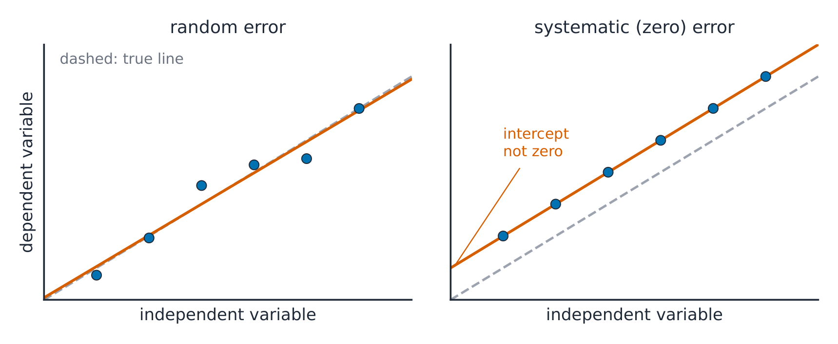
- Random effects produce unpredictable differences about an underlying mean, which may itself be biased. Systematic effects produce a consistent bias under the measurement conditions. Examples include a fixed balance offset, a scale-factor calibration error, or a heat-loss effect that changes with temperature. Systematic error need not be the same additive amount at every reading.
- In the left illustration, random scatter changes the fitted line slightly. In the right, an additive dependent-variable zero error shifts the intercept without changing the slope. A multiplicative error changes the slope; an independent-variable offset can change the intercept. Therefore a near-zero intercept does not certify that every systematic error is absent.
Does a zero-compatible intercept rule out systematic error?
Difficulté 1/5 · 100 pièces + un petit bonus lors de la première réussite aujourd'hui
The error mechanism determines which fitted quantities change.
Compare accuracy and precision
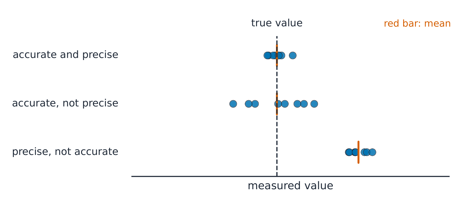
- Accuracy means closeness to the true or accepted reference value; precision concerns the closeness of repeated results. A tight cluster can be inaccurate because of a shared bias. A broad cluster may have a mean near the reference by chance, so the average and its uncertainty matter as well as the appearance of the points.
- Reliability concerns consistency when a method is repeated. Validity concerns whether it answers the intended question under appropriate controls and assumptions. A repeatable measurement of the string alone is not a valid measure of pendulum length if the model requires pivot-to-centre distance. Explain the definition, reference and method rather than labelling an entire investigation “accurate” without evidence.
Which observation can be precise but inaccurate?
Difficulté 1/5 · 100 pièces + un petit bonus lors de la première réussite aujourd'hui
Precision concerns spread; a shared bias can shift the whole cluster.
Propagate small separate bounds
- For a sum or difference, the simple maximum-uncertainty estimate adds absolute bounds. For a product or quotient, add fractional bounds. For $y=a^n$, the fractional contribution is $|n|\Delta a/|a|$. Constants defined exactly do not add measurement uncertainty. These are first-order estimates for small relative uncertainties, not universal rules for every statistical uncertainty model.
- Identify shared errors before treating contributions as separate. The very same reading subtracted from itself is exactly zero, so its uncertainty does not double. Independent standard uncertainties can be combined by statistical rules different from worst-case addition. In this course's worked bound estimates, state the approximation and keep positive uncertainty magnitudes even for a negative measured quantity.
What is x − x when both symbols refer to the very same recorded reading?
Difficulté 1/5 · 100 pièces + un petit bonus lors de la première réussite aujourd'hui
Blind separate-bound addition ignores complete correlation in this example. Distinguish the same reading from two independent readings of nominally equal quantities.
Work a quotient without early rounding
- With $V=6.0\pm0.1$ V and $I=0.25\pm0.01$ A, $R=V/I=24\ \Omega$. The fractional estimate is $0.1/6.0+0.01/0.25=0.056666\ldots$, giving $\Delta R=1.36\ \Omega$. Report $24.0\pm1.4\ \Omega$ with two uncertainty figures or $24\pm1\ \Omega$ with one.
- For a trolley travelling $1.50\pm0.01$ m in $0.62\pm0.02$ s, the unrounded speed is $2.41935\ \dfrac{\mathrm{m}}{\mathrm{s}}$. Its fractional bound is 0.0389247, so the absolute uncertainty is $0.09417\ \dfrac{\mathrm{m}}{\mathrm{s}}$. Reporting $2.42\pm0.09\ \dfrac{\mathrm{m}}{\mathrm{s}}$ keeps decimal places consistent; rounding each intermediate fraction too early can change that final uncertainty.
Use V = 6.0 ± .1 V and I = .25 ± .01 A. Find the unrounded first-order maximum absolute uncertainty in R = V/I.
Difficulté 2/5 · 140 pièces + un petit bonus lors de la première réussite aujourd'hui
R = V/I = 6.0/0.25 = 24 Ω. For the first-order maximum bound, ΔR/R ≈ ΔV/V + ΔI/I = 0.1/6.0 + 0.01/0.25 = 0.0166667 + 0.0400000 = 0.0566667. Thus ΔR ≈ 24 × 0.0566667 = 1.36 Ω, using unrounded fractions. This sums small fractional bounds, rather than combining standard uncertainties statistically.
Distance is 1.50 ± .01 m and time .62 ± .02 s. Find the first-order percentage uncertainty in speed.
Difficulté 2/5 · 140 pièces + un petit bonus lors de la première réussite aujourd'hui
For v = s/t, the first-order fractional bound is δv/v ≈ δs/s + δt/t = 0.01/1.50 + 0.02/0.62 = 0.00666666… + 0.03225806… = 0.03892473… . Multiply by 100 to obtain 3.89247…%. Each uncertainty is first divided by its own measured quantity, giving dimensionless fractions. Adding 0.01 and 0.02 directly would combine metre and second bounds incorrectly.
Find which measurement dominates
- For a cube of mass $85.2\pm0.1$ g and side $3.20\pm0.01$ cm, volume is $32.768\ \mathrm{cm^3}$ and density is $2.60010\ \dfrac{\mathrm{g}}{\mathrm{cm^3}}$. In $\rho=m/a^3$, the fractional bound is $0.1/85.2+3(0.01/3.20)=0.0105487$, giving about $0.02743\ \dfrac{\mathrm{g}}{\mathrm{cm^3}}$.
- Report $2.60\pm0.03\ \dfrac{\mathrm{g}}{\mathrm{cm^3}}$. The length contribution, 0.9375%, dominates the mass contribution, about 0.1174%. Improving the balance while leaving side measurement unchanged gives little gain. This is a reasoned improvement tied to the mathematical model, rather than a generic request for “more accurate equipment”.
For m = 85.2 ± .1 g and a = 3.20 ± .01 cm, use density m/a³. Find its first-order maximum percentage uncertainty.
Difficulté 2/5 · 140 pièces + un petit bonus lors de la première réussite aujourd'hui
For ρ = m/a³, the first-order fractional bound is δρ/ρ ≈ δm/m + 3δa/a = 0.1/85.2 + 3(0.01/3.20) = 0.00117370… + 0.009375 = 0.01054870… . Multiplying by 100 gives 1.05487…%. The power three multiplies the fractional edge-length contribution; it does not mean cubing the uncertainty. This is a first-order bound estimate for small relative uncertainties.
Preserve the raw record
- Record raw readings before processing, including units, instrument limits, repeated trials and relevant qualitative observations such as a drifting sensor or changing amplitude. Give column headings with quantity and unit; keep resolution-consistent decimal places rather than silently replacing readings with rounded processed values. Label calculated columns and show a sample calculation so the processing is reproducible.
- Continuous variables such as length can take intermediate values; counts are discrete. Choose a display to match the evidence: a scatter graph tests a relationship between numerical variables, a histogram groups a distribution, and bars compare categories. Do not join every experimental point as though each fluctuation defines the physical relationship. Keep a record of anomalies and their investigation.
Plot a test of the model
- Put the chosen independent variable horizontally and the dependent variable vertically, label quantities and units, and use a scale that makes the pattern and uncertainty visible. Draw uncertainty bars where justified; include both axes when both uncertainties matter. A best-fit line represents the overall model, rather than being forced through the origin or every point without justification.
- Statistical bars do not require every observation to touch the line. For the classroom compatible-line method, however, test possible straight lines against every specified bar or uncertainty rectangle. If none can intersect them all, inspect the model, uncertainty estimates and suspect points; do not silently enlarge bars or delete a point merely to make the theory look correct.
Check limiting gradients against all bars
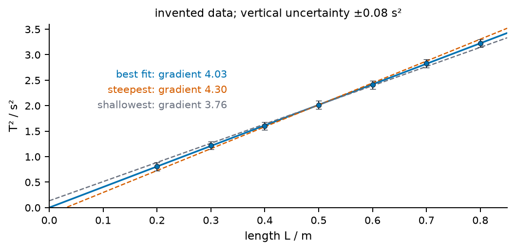
- The illustrated invented values use lengths 0.20–0.80 m, vertical bounds $\pm0.08\ \mathrm{s^2}$ and negligible horizontal uncertainty. Their best-fit gradient is $4.03\ \dfrac{\mathrm{s^2}}{\mathrm{m}}$. The limiting compatible slopes are about 4.297 and $3.763\ \dfrac{\mathrm{s^2}}{\mathrm{m}}$. Both are checked against intermediate bars; endpoint geometry alone cannot guarantee compatibility in an arbitrary dataset.
- Half their difference is about $0.267\ \dfrac{\mathrm{s^2}}{\mathrm{m}}$, or 6.6% using unrounded slopes. Rounding the extreme slopes to 4.30 and 3.76 first gives 0.27 and 6.7%, an acceptable displayed approximation here. Use a large triangle on the fitted line for the slope and divide vertical by horizontal units. Gradient uncertainty is not the same as uncertainty in each individual point.
An endpoint-to-endpoint candidate steep line misses an intermediate uncertainty bar. What should you do?
Difficulté 1/5 · 100 pièces + un petit bonus lors de la première réussite aujourd'hui
The compatible-line construction concerns every specified uncertainty bar or rectangle.
Infer gravity and interpret the intercept
- For a small-angle simple pendulum, $T^2=(4\pi^2/g)L$. With gradient 4.03 and uncertainty 0.27 in $\dfrac{\mathrm{s^2}}{\mathrm{m}}$, $g=4\pi^2/4.03=9.7961\ \dfrac{\mathrm{m}}{\mathrm{s^2}}$. The first-order relative uncertainty carries through the reciprocal, giving about $0.66\ \dfrac{\mathrm{m}}{\mathrm{s^2}}$, or $9.8\pm0.7\ \dfrac{\mathrm{m}}{\mathrm{s^2}}$ after rounding.
- In this symmetric example the limiting slope lines have intercepts near $\mp0.133\ \mathrm{s^2}$, consistent with zero. That supports proportionality within the tested range; it neither proves exact proportionality nor excludes a scale-factor error. In a general dataset, lines with extreme slopes need not have the most extreme intercepts. Determine the intercept range separately when the task requires it.
For a T² against L gradient 4.03 s²/m, use g = 4π²/gradient. Find g before rounding to its final uncertainty.
Difficulté 2/5 · 140 pièces + un petit bonus lors de la première réussite aujourd'hui
4π²/4.03 = 9.79613 m/s². Gradient units s²/m invert to m/s².
Linearise with a physical reason
- For $s=at^2/2$ with zero initial speed, plot $s$ against $t^2$; slope is $a/2$, not $a$. For $F=k/r^2$, plot $F$ against $1/r^2$; slope is $k$. The straight-line form follows from the model's assumptions. An arbitrary transformation that looks straight does not establish the intended mechanism, and non-zero initial speed would change the displacement model.
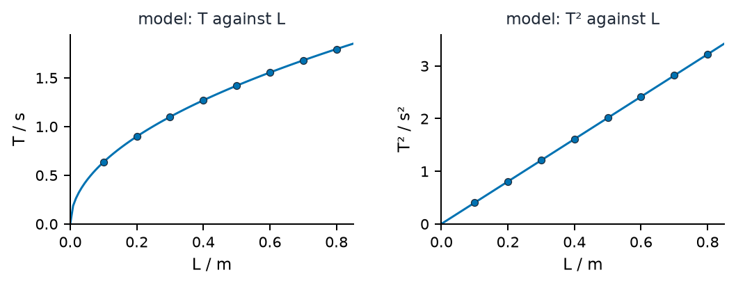
- The illustrated pendulum curves are model-generated, not independent measurements confirming the model. A plot of $T^2$ against $L$ is predicted to be straight. Transform uncertainties too: for small errors $\Delta(T^2)\approx2T\Delta T$. A fixed timing uncertainty therefore does not give the same absolute uncertainty in every squared-period point.
For s = at²/2 with zero initial speed, what does the slope of s against t² represent?
Difficulté 1/5 · 100 pièces + un petit bonus lors de la première réussite aujourd'hui
The coefficient of the plotted horizontal variable t² is a/2. The model would need an extra initial-velocity term if the start speed were not zero.
Use logarithms of dimensionless ratios
- Exponential decay gives $\ln(A/A_\mathrm{ref})=\ln(A_0/A_\mathrm{ref})-\lambda t$ for fixed positive reference activity. Plot the logarithmic ratio against time to obtain slope $-\lambda$. A raw count total must be corrected and related to activity under appropriate measurement conditions first. Zero or negative corrected values cannot simply be logged.
- For $y=kx^n$, plotting $\ln(y/y_\mathrm{ref})$ against $\ln(x/x_\mathrm{ref})$ gives slope $n$ and intercept $\ln(kx_\mathrm{ref}^n/y_\mathrm{ref})$. Changing reference units changes the intercept, not the exponent. Logarithmic axes advance by equal factors rather than equal additions. Read the tick labels before calculating ratios or claiming that equal visual spacings represent equal numerical differences.
A plot of ln(A/Aref) against t has slope −.12 per second under an exponential-decay model. What is λ?
Difficulté 1/5 · 100 pièces + un petit bonus lors de la première réussite aujourd'hui
The exponential slope is −λ. The logarithm is of a positive dimensionless activity ratio.
Inspect residuals and the tested range
- A residual is observed minus predicted value. Residuals with a curved pattern suggest that a straight-line model misses structure; a drift with trial order suggests a changing condition. One distant point is a reason to check the record, apparatus and repeat measurement, not automatic permission to erase it. Explain any exclusion and consider its effect on the conclusion.
- Interpolation estimates inside the measured range. Extrapolation assumes that the model continues outside it, where new effects can matter. A large correlation coefficient does not prove causation: for example, wire temperature might rise as current is changed. Distinguish what the sampled evidence supports from a universal claim, and name an alternative explanation or untested condition when relevant.
What is an appropriate response to a suspected outlier?
Difficulté 1/5 · 100 pièces + un petit bonus lors de la première réussite aujourd'hui
Check the raw record, conditions and repeat evidence. A reasoned exclusion differs from concealing disagreement.
Design a controlled investigation
- An investigable question might ask how constantan-wire length from 0.10 to 1.00 m affects resistance while material, diameter and temperature are controlled. Measure resistance from potential difference and current, use low current, and switch off between trials to limit heating. State how each control is implemented and why it matters; merely listing “temperature” does not control it.
- Pilot the method to choose a safe range with changes larger than the measurement uncertainty. Several distinct settings and repeat readings help separate trend from scatter; five or more settings can be a starting plan, not a universal assessment minimum. Explain spacing and number from the expected relationship, available time and dominant limitations. Randomise order or check a return setting when drift could bias a trend.
Why limit current when measuring how a metal wire’s resistance depends on length?
Difficulté 1/5 · 100 pièces + un petit bonus lors de la première réussite aujourd'hui
Temperature can change resistance. Use an explicit method to keep it stable and consider remaining heating.
Use sensors without assuming perfection
- Sensors and light gates remove the human start–stop reaction contribution, but retain response time, sampling, calibration and triggering limits. A card of known length through a gate gives length divided by interruption time: an average speed over that passage, approximating instantaneous speed only when speed changes little. A temperature sensor needs time to approach the temperature of its surroundings.
- In motion video, put a scale in the plane of motion, view square-on, and check frame timing. A scale farther from the camera than the moving object gives a perspective error. Spreadsheet formulas should reference the intended cells, retain units and avoid unintended early rounding. Software regression does not by itself validate the physical model or supply all instrument uncertainty.
Does replacing a handheld stopwatch with a sensor remove every timing limitation?
Difficulté 1/5 · 100 pièces + un petit bonus lors de la première réussite aujourd'hui
The human reaction contribution may be removed while other uncertainty mechanisms remain.
Evaluate databases and simulations
- For database evidence, record source, units, selection criteria, exclusions and uncertainty information. A catalogue selected by apparent brightness can under-represent faint objects; an observed sample relationship may therefore depend on selection. Match quantities from compatible conditions and dates rather than combining columns solely because their names look similar.
- A simulation exposes consequences of its rules and parameter choices. Vary a controlled parameter, document settings and resolution, and inspect numerical sensitivity. Data generated by the same assumed equation cannot independently prove that equation describes nature. Distinguish measurement uncertainty, sampling limitations and model limitations; repeating a deterministic simulation with unchanged settings may add no new evidence.
A deterministic simulation uses T = 2π√(L/g). Does its perfectly straight T²–L graph independently establish the law in nature?
Difficulté 1/5 · 100 pièces + un petit bonus lors de la première réussite aujourd'hui
A model-generated dataset can test implementation and explore predictions, but not independently validate its own physical assumptions.
Link safety to the actual method
- Identify the hazard, exposure route and practical control: secure falling masses, protect against hot liquid, use suitable low-voltage apparatus, and prevent direct or reflected laser exposure under the school protocol. Radioactive-source work uses teacher-approved procedures, handling tools, limited time, distance and source-appropriate shielding and storage. “Use lead” is not a universal instruction for every radiation type.
- Consider privacy or consent where people contribute data, and avoid unnecessary environmental waste or energy use. Record how the chosen controls allow the research question to be answered safely. These are method choices, not a decorative risk list detached from the equipment. If a proposed range is unsafe or outside a sensor's specification, revise the investigation before collecting it.
Compare with a reference fairly
- Percentage error is $100|x-x_\mathrm{ref}|/|x_\mathrm{ref}|$ for a non-zero reference. It is different from percentage uncertainty. For invented $g=9.2\pm0.3\ \dfrac{\mathrm{m}}{\mathrm{s^2}}$ and reference 9.81 with negligible uncertainty, the percentage difference is about 6.22%; the interval 8.9–9.5 excludes the reference under the stated estimate.
- This discrepancy does not uniquely prove a calibration fault. Check the uncertainty model, random variation, measurement definition and physical assumptions. Measuring the pendulum length too short would bias $g=4\pi^2L/T^2$ low. If a reference has appreciable uncertainty, include that too before assessing compatibility. Agreement is evidence of consistency, not proof that all errors vanished.
A measured g is 9.2 m/s² and reference is 9.81 m/s². Find percentage error using a negligible reference uncertainty.
Difficulté 2/5 · 140 pièces + un petit bonus lors de la première réussite aujourd'hui
Absolute discrepancy = |g − gref| = |9.2 − 9.81| = 0.61 m/s². Percentage error = 100|g − gref|/|gref| = 100 × 0.61/9.81 = 6.21814%. The reference value supplies the denominator. This percentage error differs from the reported measurement uncertainty.
If pendulum length is measured to the top of the bob instead of its centre, what bias is expected in g = 4π²L/T² with correct T?
Difficulté 1/5 · 100 pièces + un petit bonus lors de la première réussite aujourd'hui
In this formula g is proportional to the measured L. Correct the operational definition rather than expecting repeats to cancel it.
Write a conclusion that follows the evidence
- Answer the research question with a quantified relationship, range and uncertainty: for example, the squared period is compatible with proportionality to length over the tested interval under a small-angle model. Quote the fitted constant and compare it with a justified reference. Keep original observations distinct from processed data and theory.
- Evaluate specific limitations by mechanism, direction and size where possible. If timing dominates, a light gate or longer timing interval can help; if a length definition is biased, correct that definition. If temperature drift changes resistance, reduce heating or measure temperature. An improvement is strongest when you explain which uncertainty or bias it reduces and why that matters for the conclusion.
Design and evaluate a pendulum investigation that uses T² against L to infer g, distinguishing measurement, processing, compatibility and model limitations.
Connect the evidence chain from operational definitions to a conclusion with assumptions and a targeted evaluation.
Plan the individual scientific investigation
- The scientific investigation is common to SL and HL: 20% of the final grade, about ten teaching hours and a report of at most 3000 words. The four six-mark criteria concern research design, data analysis, conclusion and evaluation. Quantitative evidence can come from appropriate experiments, fieldwork, databases, simulations or modelling; the question must support meaningful analysis rather than a descriptive summary alone.
- Consult the IB Physics guide for details, including word-count exclusions. Optional groups have at most three students, with individual questions, distinct data or suitable distinct subsets, and individually authored reports. Cite sources and identify simulated data honestly. The interdisciplinary collaborative sciences project is separate from this individual assessment.