Do Those Points Align? (Extension)
Introducido| English | Significado |
|---|---|
| least-squares regression/liːst skweəz rɪˈɡreʃn/ | regresión de mínimos cuadrados |
The slope wobbles too
- In Unit 2 we fit a least-squares line and read its slope $b$.
- But $b$ comes from a sample — a different sample can give a different slope.
- So the slope varies from sample to sample, just like $\bar{x}$ or $\hat{p}$.
- Unit 9 does inference about the true slope $\beta$ behind the data; slope inference is extension content beyond the revised AP exam.
The sampling distribution of b
- Collect the slope $b$ from every possible sample → its sampling distribution.
- Under a linear model with independent errors of mean zero at each $x$, $b$ is centered at the true population slope $\beta$ (unbiased conditional on the $x$ values).
- The standard error of the slope, $SE_b$, estimates the spread of $b$; it is not the exact unknown sampling SD.
- For independent normal errors with constant SD, $(b-\beta)/SE_b$ has a $t$-distribution with $n-2$ degrees of freedom; the raw $b$ does not.
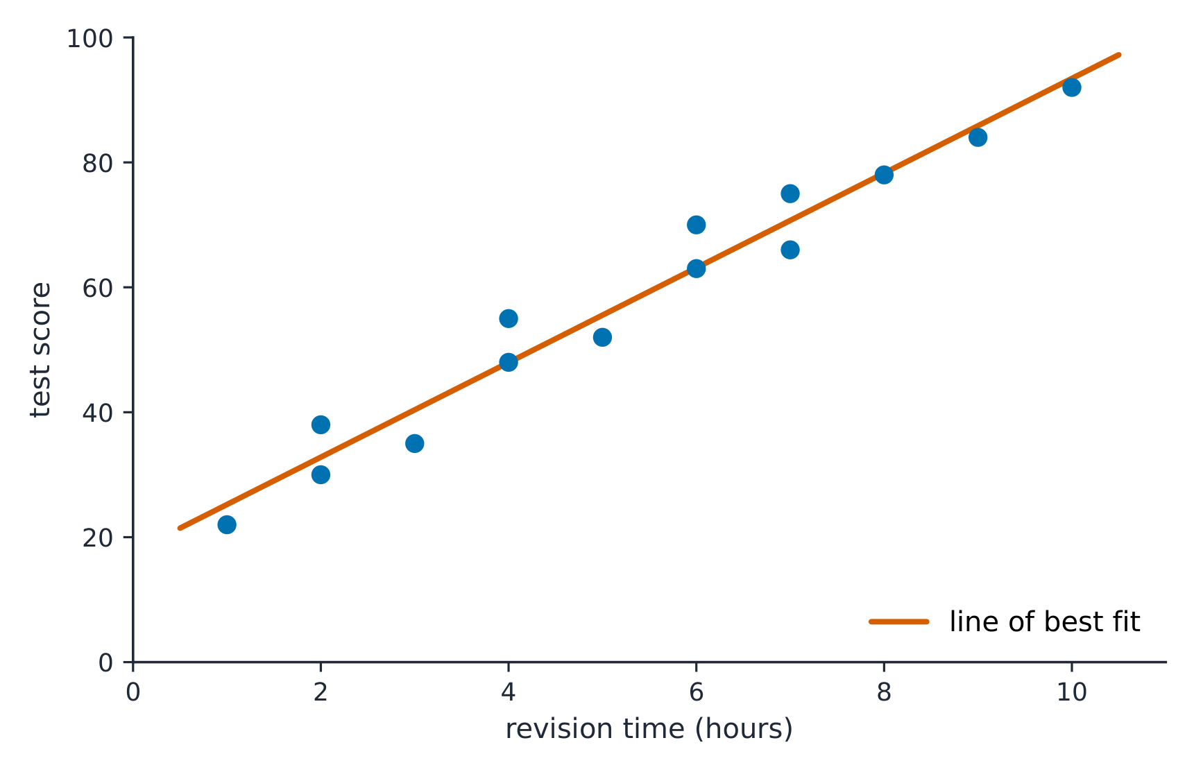
A line of best fit runs through the middle of the scattered points
Inference about the relationship
- Inference for slopes asks: is there really a linear relationship, and how strong?
- The true slope $\beta$ is unknown; $b$ estimates it with uncertainty.
- A confidence interval gives a range for $\beta$; a test judges whether $\beta = 0$.
- Both quantify how sure we are about the line behind the scatter.
Built on Unit 2
- Everything rests on the least-squares regression 最小二乘回归 model $\hat{y} = a + bx$.
- $b$ is still the predicted change in $y$ per unit $x$ — now with error bars.
- We add a $t$-based interval and test around that slope.
- Regression inference is "Unit 2's slope, plus Unit 7's $t$-machinery."
The slope $b$ from one sample is an estimate, not the truth $\beta$. A different random sample can give a different $b$. Inference for slopes is exactly the same logic as for means — a $t$-based interval and test around a sample statistic — applied to the regression slope, with its own standard error $SE_b$.
Fitting hours-studied vs. score for one class gives slope $b = 4.2$.
- Another random sample from the same target population could give $b=3.8$ or $4.6$ — sampling variability.
- The true slope $\beta$ for the sampled population is unknown; $b = 4.2$ estimates it.
- Unit 9 builds an interval and a test for that unknown $\beta$.
The slope $b$ of a fitted line varies from sample to sample; under the linear-model assumptions, it is unbiased for $\beta$, and $SE_b$ estimates its spread. The standardized statistic $(b-\beta)/SE_b$, rather than raw $b$, follows a $t$-distribution under independent normal errors with constant SD. Inference for slopes quantifies the uncertainty about the true linear relationship, building directly on the least-squares regression model.
Write from this case
- Many random samples are taken from one linear relationship.
- Each sample has its own least-squares slope.
Repeated random samples from one fixed linear population relationship give different least-squares slopes. Why can they differ?
A new random sample can produce a different fitted slope through sampling variability, while the population slope remains fixed.
What varies across samples?
Dificultad 1/5 · 100 monedas + un pequeño bono en el primer intento de hoy
Sample slopes differ. The population slope is fixed.
A fitted slope varies by sample
Each sample's least-squares line has a slightly different slope b.
The slope b from a sample is...
Dificultad 1/5 · 100 monedas + un pequeño bono en el primer intento de hoy
b estimates the unknown population slope β, with uncertainty.
Under the linear regression model with independent mean-zero errors conditional on x, the sample slope b is unbiased for β.
Dificultad 1/5 · 100 monedas + un pequeño bono en el primer intento de hoy
b is unbiased for β.
With independent normal errors of constant SD, which reference distribution applies to (b − β)/SE_b?
Dificultad 1/5 · 100 monedas + un pequeño bono en el primer intento de hoy
The standardized slope statistic follows t with n − 2 degrees of freedom; this does not mean the raw slope b has a t distribution.
Regression inference builds on the least-squares model ŷ = a + bx from Unit 2.
Dificultad 1/5 · 100 monedas + un pequeño bono en el primer intento de hoy
It adds a t-interval and test around the Unit 2 slope.
The estimated sampling spread of b is the standard error of the ___ (one word).
Dificultad 1/5 · 100 monedas + un pequeño bono en el primer intento de hoy
SE_b is the standard error of the slope.