Uncertainty, gradients and model testing
Introduzido| English | Significado |
|---|---|
| systematic error/ˌsɪstəˈmætɪk ˈerə/ | erro sistemático |
| uncertainty/ʌnˈsɜːtənti/ | incerteza |
What would explain this observation?
- A line passing near every data point is useful, but its gradient can still be uncertain. A graph is evidence for a model within the measurement range.
Build the model
- Random variation makes repeated readings differ.
- Systematic error 系统误差 shifts results consistently.
- Absolute uncertainty 不确定度 has the measured unit; relative or percentage uncertainty compares uncertainty with the measured value.
- uncertainty: A quantified limitation on a measured result.
- systematic error: A consistent measurement bias.

Which is most likely a systematic error?
Dificuldade 1/5 · Moedas 100 + pequeno bônus na primeira conclusão hoje
A fixed 0.20 g balance zero offset is a systematic error. Independent repeats reduce random uncertainty in the mean, not scatter in individual readings or a shared offset. Reaction timing can have both random and systematic contributions.
Match each technical term to its precise meaning.
Dificuldade 2/5 · Moedas 140 + pequeno bônus na primeira conclusão hoje
Use the definitions to distinguish related quantities and processes.
Choose evidence that can test it
- For a product or quotient, adding fractional uncertainties is a common maximum-uncertainty approximation.
- For a difference, add absolute uncertainties.
- A nonzero intercept can reveal an offset or an incomplete model.
In the lab: Show units on axes and choose a sensible scale. Plot uncertainty bars where justified, draw a best-fit line rather than joining every point, and estimate steepest and shallowest plausible gradients when the course method calls for them.
Which two habits make the investigation or model in this case more defensible?
Dificuldade 2/5 · Moedas 140 + pequeno bônus na primeira conclusão hoje
Stating the conditions and assumptions lets others repeat the work exactly, and recording the supporting evidence lets them check the conclusion. Hiding disagreeing results removes the evidence that could challenge a wrong conclusion, and one measurement can never establish a wider claim.
Work from known quantities
- Known: length = 50.0 mm with uncertainty 1.0 mm.
- Percentage uncertainty = absolute uncertainty/value ×100 = 1.0/50.0×100 = 2.0%.
- For a quotient of two independently measured quantities with maximum percentage uncertainties 2% and 3%, the summed maximum estimate is 5%.
Your turn: A 40 cm reading has an absolute uncertainty of 1 cm. Find percentage uncertainty.
Measurement ranges and the quotient estimate
50 ± 1 mm has a 2% uncertainty. Compare it with a 100 ± 3 mm reading: the summed quotient estimate is 5%, while exact endpoint calculations reveal a slightly asymmetric range.
A 40 cm reading has an absolute uncertainty of 1 cm. Find percentage uncertainty.
Dificuldade 2/5 · Moedas 140 + pequeno bônus na primeira conclusão hoje
The result is 2.5 %. Known: reading 40 cm; absolute uncertainty 1 cm. Use percentage uncertainty = absolute uncertainty / value x 100. Percentage uncertainty = 1/40 x 100 = 2.5%. Smaller measured values carry larger percentage uncertainties for the same absolute uncertainty.
Check the conclusion and its limits
- Repeating readings reduces random uncertainty in a mean but does not automatically remove a zero error.
- Do not quote more decimal places than your measurement can support.
Not true: Repeating a measurement always removes a calibration offset. Independent repeats and averaging can reduce random uncertainty of the mean, while a calibration offset can remain. Check calibration and apply a justified correction where appropriate.
- Random variation makes repeated readings differ.
- For a product or quotient, adding fractional uncertainties is a common maximum-uncertainty approximation.
- Watch for: repeating readings reduces random uncertainty in a mean but does not automatically remove a zero error.
Repeating a measurement always removes a calibration offset.
Dificuldade 1/5 · Moedas 100 + pequeno bônus na primeira conclusão hoje
Independent repeats and averaging can reduce random uncertainty of the mean, while a calibration offset can remain. Check calibration and apply a justified correction where appropriate.
A quantified limitation on a measured result: write the technical term.
Dificuldade 1/5 · Moedas 100 + pequeno bônus na primeira conclusão hoje
uncertainty means A quantified limitation on a measured result.
A reading is 25 cm and the absolute uncertainty is 2 cm. What is the percentage uncertainty, and what does repeating the measurement not remove?
Percentage uncertainty = absolute uncertainty/measured reading × 100 = 2/25 × 100 = 8%. Independent repeats and averaging can reduce random uncertainty of the mean; they do not remove a shared calibration offset. Check calibration and apply a justified correction where appropriate.
A reading is 25 cm with an absolute uncertainty of 2 cm. What is its percentage uncertainty?
Dificuldade 1/5 · Moedas 100 + pequeno bônus na primeira conclusão hoje
2/25 × 100 = 8%. This is the written case. The earlier separate 40 cm reading with 1 cm uncertainty gives 2.5%, not the answer to this case.
Write from a measured value and its uncertainty
- In the original written case, a 25 cm reading has absolute uncertainty 2 cm. Percentage uncertainty is $2/25\times100=8\%$. This differs from the earlier 40 cm, 1 cm case, which gives 2.5%. Always attach an answer to its own measurements. Repetition does not automatically remove a calibration offset shared by all readings.
- The following original, invented investigations develop shared SL/HL experimental skills. Plan a measurable question, choose apparatus, preserve raw data, process uncertainty and evaluate the resulting claim. Numerical uncertainty values are supplied for these examples; they are not universal specifications for every instrument of that type.
Turn a broad topic into a measurable question
- “How does temperature affect chemistry?” does not define a measurement. A narrower example asks how initial temperature changes the time for a specified magnesium strip to produce 20 cubic centimetres of hydrogen in a fixed hydrochloric acid mixture. Temperature is the independent variable; elapsed time is dependent. For a fixed collected volume, $1/t$ compares average rates, not automatically initial rates.
- Explain controls: acid concentration changes collision conditions, exposed magnesium area changes contact with acid, and a leak changes collected gas without measuring a slower reaction. Choose a supervised range and use a pilot trial to identify reactions too fast to time. Repeated trials estimate scatter; they do not replace testing several values of the independent variable.
Match the instrument to the operation
- A volumetric pipette delivers a specified volume; a burette delivers a variable volume from a difference of readings; a volumetric flask contains a specified total volume at its mark. To dilute 20.0 cubic centimetres of a stock solution to 100.0, add solvent until the final mixture reaches the mark. Adding 100.0 of solvent would give the wrong final volume.
- For an invented stock concentration $0.500\ \dfrac{\mathrm{mol}}{\mathrm{dm}^3}$, conserving solute gives $c_2=0.500\times20.0/100.0=0.100$ in the same units. Dissolve and transfer quantitatively, rinse the original vessel into the flask and mix thoroughly. A precise balance reading cannot compensate for impure material or solute left behind during transfer.
Read the burette as a difference
- Burette values increase downwards. For a suitable clear solution with a concave meniscus, read its bottom at eye level and record both readings. In the invented case, initial 2.35 and final 24.85 cubic centimetres give $24.85-2.35=22.50$ delivered. The initial value need not be zero; a bubble in the tip can still compromise delivery.
- If each reading has stated maximum uncertainty 0.05 cubic centimetres, add absolute uncertainties for the difference: $0.05+0.05=0.10$. The result is $22.50\pm0.10\ \mathrm{cm}^3$. The uncertainty does not subtract just because the volume readings subtract. Readings from the same instrument may nevertheless share a constant zero offset that cancels in the difference.
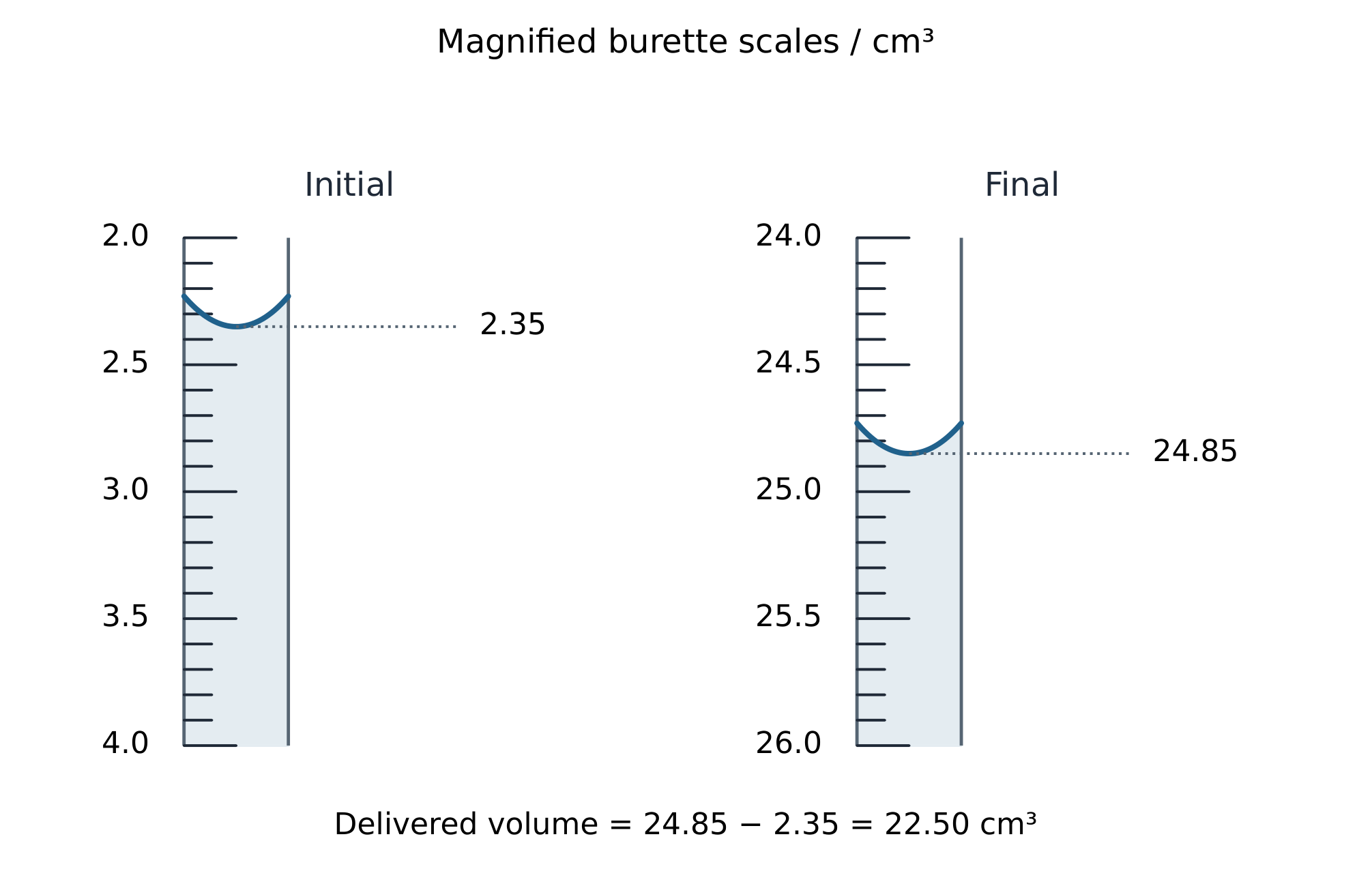
A burette initially reads 2.35 cubic centimetres and finally 24.85. What volume was delivered?
Dificuldade 2/5 · Moedas 140 + pequeno bônus na primeira conclusão hoje
Final minus initial: 24.85 − 2.35 = 22.50 cubic centimetres. Burette readings increase downwards; the initial reading need not be zero.
Separate precision, accuracy and repetition
- An invented 25.00 g reference produces readings 25.20, 25.21 and 25.19 g. Their mean is 25.20 g and their range is only 0.02 g. The readings agree closely but are biased high relative to the reference. Small scatter describes precision; it does not prove accuracy. Additional repeats around the same offset do not remove that offset.
- Calibrate against an appropriate reference, and match reference conditions to the measurement. Randomizing condition order can reduce confusion from gradual drift; it does not fix every bias. A gas leak or heat loss can have a directional effect without behaving like a constant zero error. Name the physical mechanism before deciding which improvement would address it.
Propagate uncertainty using one stated method
- In the conservative maximum method, add absolute uncertainties for sums and differences; add fractional uncertainties for products and quotients. For $y=a/b$, estimate $u_y/|y|\approx u_a/|a|+u_b/|b|$. This is a small-uncertainty, first-order estimate. Do not switch to a statistical combination rule halfway through the same answer.
- An exact conversion or defined stoichiometric coefficient adds no measurement uncertainty. Multiplying a measured value by exactly two doubles its absolute uncertainty but leaves its percentage uncertainty unchanged. A statistical standard uncertainty and a conservative maximum range describe different things; correlated readings may need separate treatment rather than automatic independent-error combination.
Carry the uncertainty into a chemical result
- An invented 1:1 titration uses $25.00\pm0.03\ \mathrm{cm}^3$ of alkali and $22.50\pm0.10\ \mathrm{cm}^3$ of acid. The acid concentration is $0.1000\ \dfrac{\mathrm{mol}}{\mathrm{dm}^3}$ with 0.20% uncertainty. Alkali concentration is $0.1000\times22.50/25.00=0.09000$ in the same concentration units. The volume ratio needs no conversion because both volumes use the same unit.
- Maximum percentage uncertainty is $0.20+100(0.10/22.50)+100(0.03/25.00)\approx0.764\%$. Absolute uncertainty is $0.09000\times0.00764\approx0.00069$ in the concentration unit. A suitable rounded report is $0.0900\pm0.0007\ \dfrac{\mathrm{mol}}{\mathrm{dm}^3}$. Keep guard digits until the end and align the reported value with the uncertainty's decimal place.
A 1:1 titration uses acid concentration 0.1000 mol/dm³ with maximum uncertainty 0.20%, titre 22.50 ± 0.10 cm³ and alkali pipette volume 25.00 ± 0.03 cm³. Add percentage contributions to find the maximum percentage uncertainty in the alkali concentration.
Dificuldade 2/5 · Moedas 140 + pequeno bônus na primeira conclusão hoje
For c(alkali) = c(acid) × titre/pipette volume, add maximum percentage contributions. Titre contributes 0.10/22.50 × 100 = 0.44444…%; pipette contributes 0.03/25.00 × 100 = 0.120%. Total = 0.20 + 0.44444… + 0.120 = 0.76444…%. The concentration is 0.1000 × 22.50/25.00 = 0.09000 mol/dm³, with absolute uncertainty 0.09000 × 0.76444…/100 = 0.000688 mol/dm³, about 0.00069.
Choose a graph that represents the measurements
- Use a scatter plot for paired continuous measurements, a bar chart for categories and a histogram for a continuous distribution grouped into intervals. Label quantities and units; select a readable scale. A quantitative axis need not always begin at zero. A qualitative sketch has labelled but unscaled axes, rather than invented numerical precision.
- Draw a justified best-fit line or curve instead of joining each noisy point. Calculate a line's gradient from two widely separated positions on that fitted line; they need not be measured data points. Gradient units are vertical-axis units divided by horizontal-axis units. A tangent estimates an instantaneous gradient; a chord estimates an average over an interval.
Use the intercept in a calibration
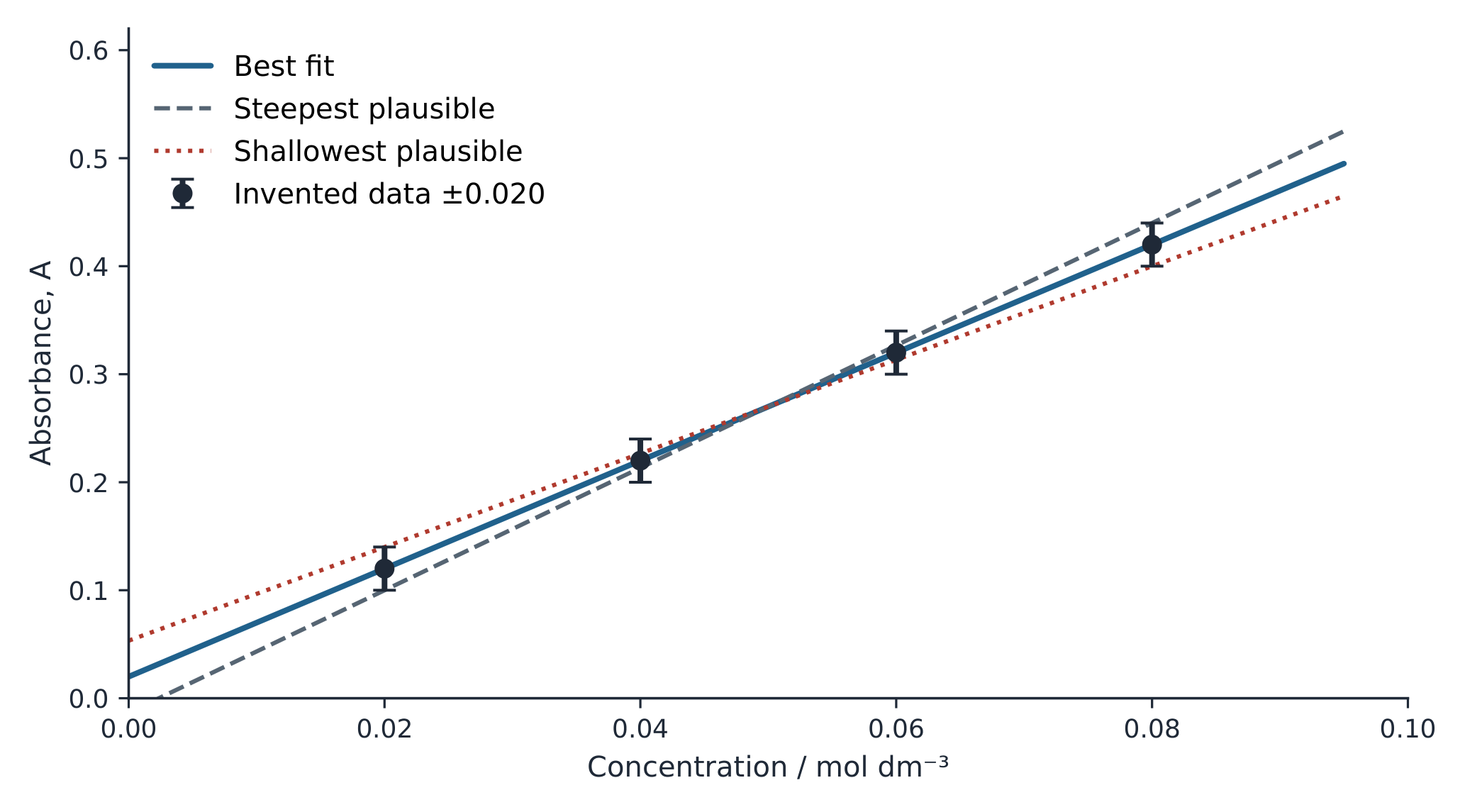
- Invented concentrations 0.020, 0.040, 0.060 and 0.080 moles per cubic decimetre give absorbances 0.120, 0.220, 0.320 and 0.420. The line is $A=5.00c+0.020$. An unknown absorbance of 0.270 gives $c=(0.270-0.020)/5.00=0.0500$ moles per cubic decimetre. Dividing 0.270 directly by 5.00 would ignore the intercept.
- Investigate a nonzero intercept as a possible blank offset, background signal or model limitation; do not force the line through zero automatically. The unknown lies inside this calibration range, so this is interpolation. An unknown well outside the standards requires additional justification or suitable dilution; extrapolation can fail when the relationship is no longer linear.
An invented calibration is A = 5.00c + 0.020, with c in mol/dm³ and standards covering 0.020 to 0.080 mol/dm³. Find c for absorbance A = 0.270.
Dificuldade 2/5 · Moedas 140 + pequeno bônus na primeira conclusão hoje
Rearrange A = 5.00c + 0.020 to c = (A − 0.020)/5.00. Substitute c = (0.270 − 0.020)/5.00 = 0.250/5.00 = 0.0500 mol/dm³. This lies between 0.020 and 0.080, so the estimate is interpolation within the stated standard range.
Constrain a gradient with the full set of uncertainty bars
- Give each absorbance above an uncertainty of 0.020 and neglect horizontal uncertainty in this model. The steepest allowed line passes through $(0.020,0.100)$ and $(0.080,0.440)$; its gradient is $0.340/0.060\approx5.67$. The shallowest passes through $(0.020,0.140)$ and $(0.080,0.400)$, giving $0.260/0.060\approx4.33$.
- Check the intermediate bars too: choosing extreme endpoint corners does not by itself establish a line consistent with all observations. Midpoint and half-range give gradient approximately $5.00\pm0.67$ cubic decimetres per mole here. This graphical range follows the stated bars and straight-line model; it is not automatically a formal statistical confidence interval or proof that the model is correct.
Distinguish techniques by what they accomplish
- Filtration separates insoluble solid from liquid; dissolved salt passes through an ordinary filter with its solvent. Distillation collects condensed vapour, whereas reflux returns condensate to the reaction vessel. Recrystallization exploits a suitable solubility difference between hot and cold solvent. Drying to constant mass uses repeated appropriate heat–cool–weigh cycles; constant mass alone does not prove chemical purity.
- In chromatography, measure the spot and solvent-front distances from the same baseline. Invented distances 3.6 and 6.0 cm give $R_f=3.6/6.0=0.60$, with no unit. Keep the initial solvent below the spot and mark its front promptly. Matching a reference's ratio under matching conditions supports comparison but does not independently establish a complete molecular identity.
From the same chromatography baseline, a spot moves 3.6 cm and the solvent front 6.0 cm. Find Rf.
Dificuldade 2/5 · Moedas 140 + pequeno bônus na primeira conclusão hoje
Spot distance divided by solvent-front distance is 3.6/6.0 = 0.60. Units cancel; the ratio alone does not establish molecular identity.
Evaluate the claim through a specific mechanism
- A high fitted $R^2$ does not prove accuracy, causation or freedom from bias. Even a perfectly straight set of readings can share a calibration error. Inspect residual patterns, range, replication and the underlying chemistry. Preserve raw readings and unexpected observations; record a justified exclusion rule rather than silently deleting a disagreeing result.
- Connect each limitation to its effect and a practical improvement. For a leaking gas collection system, lost gas lowers measured volume and can bias the inferred rate; checking connections and testing for leaks addresses that mechanism. “Use better apparatus” does not identify a cause. Link hazards to exposure routes and controls, and follow supervised apparatus limits and waste instructions throughout.
A gas-producing investigation gives repeatable low gas volumes and a strong fitted trend. Evaluate whether this proves accuracy when a connection may leak.
Evaluation needs a specific physical mechanism, its effect on the result and a relevant feasible improvement.
AHL: Propagate a power using its magnitude
- For $y=x^n$ with an exact exponent and small uncertainty, the approximate fractional uncertainty is multiplied by $|n|$. An invented 2% uncertainty in $x$ therefore gives about 4% in $1/x^2$. The negative exponent changes how the value depends on $x$, not the sign of the uncertainty. A measured uncertainty is reported as a nonnegative magnitude.
- This is a first-order approximation; large fractional uncertainties and values near singularities require care. Constants known exactly add no measurement uncertainty. State the propagation convention explicitly and retain the units of the final quantity; a compact algebraic rule does not excuse an inappropriate physical model.
AHL: Linearize an exponential without taking a logarithm of units
- In an invented concentration model, $c=c_0e^{-kt}$ with $c_0=0.1000\ \dfrac{\mathrm{mol}}{\mathrm{dm}^3}$ and $k=0.0200\ \dfrac{1}{\mathrm{s}}$. At 30.0 s, $c=0.1000e^{-0.600}\approx0.0549$ in the same concentration unit. Rearranging gives $\ln(c/c_0)=-kt$: the logarithm acts on a dimensionless ratio, and a plot against time has gradient $-k$.
- Half the initial concentration occurs when $1/2=e^{-kt}$, so the half-time is $\ln2/0.0200\approx34.7$ s. An approximately straight transformed graph supports the exponential description over the tested range. It does not uniquely establish a chemical mechanism, and a change in conditions can make extrapolation inappropriate.
AHL: An invented concentration model is c = c₀ exp(−kt), with k = 0.0200 per second. Find the time for concentration to halve.
Dificuldade 2/5 · Moedas 140 + pequeno bônus na primeira conclusão hoje
At half concentration, c/c₀ = 1/2 = exp(−kt). Taking natural logarithms gives ln(1/2) = −kt. Therefore t = −ln(1/2)/k = ln 2/0.0200 = 34.657… s, about 34.7 s. The logarithm acts on the dimensionless concentration ratio.
Choose the comparison denominator
- For an invented measured mass $10.40\pm0.10$ g and accepted reference 10.00 g, percentage uncertainty is $100(0.10/10.40)=0.96\%$. The magnitude of percentage error is $100|10.40-10.00|/10.00=4.0\%$. The first denominator is measured; the second is the reference. Small uncertainty does not establish accuracy.
- A change from 10.00 to 10.40 g is $+4.0\%$ of the initial value. For two comparable measurements with neither a reference nor an initial role, one common percentage difference uses their mean: $100(0.40/10.20)=3.92\%$. State the convention and follow any denominator specified in the question.
An invented mass measurement is 10.40 ± 0.10 g and the accepted reference is 10.00 g. Find the magnitude of percentage error.
Dificuldade 2/5 · Moedas 140 + pequeno bônus na primeira conclusão hoje
Use the accepted reference as denominator: 100 × |10.40 − 10.00| / 10.00 = 4.0%. The separate percentage uncertainty is 100 × 0.10 / 10.40 ≈ 0.96%.
Interpret the fit before evaluating the method
- For an invented calibration fitted with an intercept, $R^2=0.81$ means the model accounts for 81% of variation in the measured response within this dataset; 19% remains in residual variation. It does not mean 81% of readings are accurate or that concentration caused 81% of the variation.
- A second model with $R^2=0.94$ accounts for more of the same response variation. Check its physical meaning, residual pattern and possible calibration bias before judging the method. A shared bias can remain even when points fit a line extremely closely.
An invented calibration fitted with an intercept reports R² = 0.81. Which interpretation is justified?
Dificuldade 1/5 · Moedas 100 + pequeno bônus na primeira conclusão hoje
R² describes how much response variation the fitted model accounts for under the stated regression convention. It does not measure accuracy or prove causation; remaining residual variation is not missing measurements.