Statistics 2: distributions, continuous variables and hypothesis tests
Statistics 2 (S2, paper WST02/01, 1 hour 30 minutes, 75 marks, first assessment June 2020) follows S1 in the applied route: P1–P2 and S1 are assumed. The booklet carries the binomial, Poisson and Normal tables. This reference covers the binomial and Poisson distributions with their approximations, continuous random variables, the uniform distribution, sampling and the full hypothesis-testing routine.
Must-know for S2 (not in the booklet):
| Family | Formulae |
|---|---|
| binomial | $X\sim B(n, p)$: $E(X) = np$, $\mathrm{Var}(X) = np(1-p)$, $P(X = r) = \binom nr p^r(1-p)^{n-r}$ |
| Poisson | $X\sim\mathrm{Po}(\lambda)$: $E(X) = \mathrm{Var}(X) = \lambda$; rates scale with time |
| continuous | $P(a < X < b) = \int_a^b f(x)\,dx$, $f(x) = F'(x)$, $E(X) = \int xf(x)\,dx$, $E(X^2) = \int x^2f(x)\,dx$ |
| uniform | on $[a, b]$: mean $\tfrac{a+b}2$, variance $\tfrac{(b-a)^2}{12}$, density $\tfrac1{b-a}$ |
The binomial and Poisson distributions
Binomial distribution 二项分布: $n$ independent trials, constant probability $p$ — the two assumptions to state in context. Poisson distribution 泊松分布: events occur singly, independently, at a constant average rate — the rate scales ($\mathrm{Po}(\lambda)$ per minute gives $\mathrm{Po}(5\lambda)$ in 5 minutes). Moments come as formulas: $np$ and $np(1-p)$; $\lambda$ and $\lambda$. Given the mean and variance of a binomial, solve for $n$ and $p$ simultaneously. The Poisson approximation to the binomial needs $n$ large and $p$ small (use $\lambda = np$).
Worked example — moments then approximations (WST02 June 2025 Q3). Blue sweets per small bag have mean 3 and variance 2.55: $np = 3$ and $np(1-p) = 2.55$ give $1 - p = 0.85$, so $p = 0.15$ and $n = 20$. A medium bag of 40 with 20% green: $X\sim B(40, 0.2)$, $E(X) = 8$, and $P(X > 8) = 1 - P(X \le 8) = 0.407$. A large bag of 80 with 10% yellow: with $n = 80$ large and $p = 0.1$ small, $X\approx\mathrm{Po}(8)$ and $P(X \ge 12) = 1 - P(X \le 11) = 0.112$.
Continuous random variables
A continuous random variable has a probability density function 概率密度函数 $f$ with total area 1 and $P(X = x) = 0$ at every point; the cumulative distribution function 分布函数 $F(x) = P(X \le x)$ satisfies $f = F'$ and $F(a) = \int_{-\infty}^a f$. Piecewise densities: normalise $\int f = 1$ (which pins the unknown constant), then read off the median 中位数 ($F = \tfrac12$), quartiles, and the mode 众数 from the peak of $f$ (set $f' = 0$, or inspect corners). $E(X) = \int xf\,dx$, $E(X^2) = \int x^2f\,dx$, $\mathrm{Var} = E(X^2) - [E(X)]^2$; skewness compares mean, median and mode.
![Left: the CDF F(x) = (6x^2 - x^4)/5 on [0, 1] rising from 0 to 1 with the median marked at F = 1/2 (x = 0.671). Right: the density f(x) = (12x - 4x^3)/5 with the mode at x = 1 and the area beyond x = 0.6 shaded (0.594).](/handout-media/edexcel_ial_further_mathematics/assets/08-cdf-pdf.png?v=1792133600)
Worked example — a CDF worked through (WST02 June 2025 Q1). $F(x) = k(6x^2 - x^4)$ on [0, 1]: $F(1) = 1$ gives $5k = 1$. $P(X > 0.6) = 1 - \tfrac{6(0.36) - 0.1296}{5} = 0.594$. The median: $\tfrac{6m^2 - m^4}{5} = \tfrac12$, i.e. $2m^4 - 12m^2 + 5 = 0$, so $m = 0.671$. The mode: $f(x) = \tfrac{12x - 4x^3}{5}$ and $f'(x) = \tfrac{12 - 12x^2}{5} = 0$ gives $x = 1$ (reject $-1$, outside the support). Skewness: mean $0.64 <$ median $0.671 <$ mode $1$ — negative skew.
![Left: a triangular pdf rising along 2x/21 from 0 to k = 3.5 then falling along 2(6-x)/15 to x = 6, peak value 1/3 marked. Right: the uniform density on [-2, 14] at height 1/16 with the interval [8, 14] shaded (area 3/8).](/handout-media/edexcel_ial_further_mathematics/assets/08-triangular-pdf.png?v=1792133600)
Worked example — a piecewise-linear pdf, no calculator (WST02 June 2025 Q5). With $f(x) = \tfrac{2x}{21}$ on $[0, k]$ and $f(x) = \tfrac{2(6-x)}{15}$ on $(k, 6]$: normalising,
so $k = 3.5$ (the pdf is continuous there, both pieces equalling $\tfrac13$). Then $E(X) = \tfrac{2}{21}\cdot\tfrac{k^3}{3} + \tfrac{2}{15}\int_{3.5}^6(6x - x^2)dx = \tfrac{19}6$, and with $E(X^2) = \tfrac{277}{24}$ given, $\mathrm{Var}(X) = \tfrac{277}{24} - \tfrac{361}{36} = \tfrac{109}{72}$.
The continuous uniform distribution
The continuous uniform distribution 均匀分布 on $[a, b]$ Uniform on $[a, b]$: density $\tfrac1{b-a}$, straight CDF, mean $\tfrac{a+b}2$, variance $\tfrac{(b-a)^2}{12}$. Two facts pin $a$ and $b$ (an interval probability gives $b - a$; the mean gives $a + b$). Coding scales the mean; probabilities are lengths over $b - a$.
Worked example — uniform on a wide interval (WST02 June 2025 Q6). $P(2 < X < 5) = \tfrac3{16}$ gives $b - a = 16$; $E(X) = 6$ gives $a + b = 12$: so $a = -2$, $b = 14$ ($a = 4.4$, $b = 7.6$ also fits — but keep one root for the whole question). $E(cX + 1) = 3$ gives $c = \tfrac13$; $\mathrm{Var} = \tfrac{256}{12} = \tfrac{64}3$; $E(X^2) = \tfrac{64}3 + 36 = \tfrac{172}3$; and $P(\tfrac32X - b > a) = P(X > \tfrac{2(a+b)}3) = P(X > 8) = \tfrac{14-8}{16} = \tfrac38$.
Populations, samples and statistics
A census 普查 measures everybody (complete but costly, slow, possibly destructive); a sample 抽样 measures part (cheaper, faster, but with sampling error). The sampling frame 抽样框 lists the sampling units. A statistic 统计量 is a function of the sample values only (no unknown parameters) — $\bar X$ is, $\bar X - \mu$ is not; its distribution over repeated samples is the sampling distribution 抽样分布.
Worked example — a sampling distribution (WST02 June 2025 Q4). Three beads from a 2:5 black:white bag, scoring 4 per black and 1 per white: with $P(\text{black}) = \tfrac27$, the score $X$ takes 3, 6, 9, 12 with probabilities $\tfrac{125}{343}, \tfrac{150}{343}, \tfrac{60}{343}, \tfrac{8}{343}$ (binomial weights $\binom30(\tfrac57)^3$ etc.). If $Y$ counts 9-point sets among $n$ independent plays, $Y\sim B(n, \tfrac{60}{343})$ and $1 - (\tfrac{283}{343})^n > 0.95$ needs $n > 15.6$, so $n = 16$.
Hypothesis tests
A hypothesis test 假设检验 compares data against a null model.
State the null hypothesis 原假设 $H_0$ (no change, the quoted parameter) and $H_1$ (one- or two-tailed as asked). Find the critical region 临界域 at the stated level by accumulating tail probabilities until crossing $\alpha$; report the actual significance level 显著性水平 as the total tail probability. One-tailed tests put the whole level in one tail; two-tailed split it. Conclude IN CONTEXT: "insufficient evidence that … has changed". Normal approximations to the binomial: mean $np$, variance $np(1-p)$, with the continuity correction 连续性修正 (at least $t$ means $t - 0.5$).
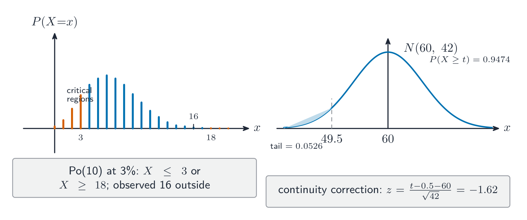
Worked example — a Poisson rate test (WST02 June 2025 Q2). Customers average 20/hour; after alterations one 30-minute interval is watched: $X\sim\mathrm{Po}(10)$, $H_0\colon\lambda = 10$, $H_1\colon\lambda \ne 10$. At 3%: $P(X \le 3) = 0.0103$ but $P(X \le 4) = 0.0293$ (too big); $P(X \ge 17) = 0.0270$ but $P(X \ge 18) = 0.0143$ — critical region $X \le 3$ or $X \ge 18$, actual level $0.0103 + 0.0143 = 2.46\%$. The observed 16 lies outside → do not reject $H_0$.
Worked example — binomial test with a Normal middle (WST02 June 2025 Q7). 30% of customers take insurance; a sample of 40 gives $X\sim B(40, 0.3)$. Largest $r$ with $P(X < r) < 0.05$ (fewer than $r$): $P(X \le 6) = 0.0238 < 0.05$ but $P(X \le 7) = 0.0553 > 0.05$, so $r = 7$. For 200 customers, $B(200, 0.3)\approx N(60, 42)$: $P(X \ge t) = 0.9474$ means $\tfrac{t - 0.5 - 60}{\sqrt{42}} = -1.62$, so $t = 50$. After a special offer, 11 of 25 buy: $H_0\colon p = 0.3$, $H_1\colon p > 0.3$; $P(X \ge 11) = 0.0978 < 0.10$, so reject $H_0$ — evidence the proportion has increased.
Checklist before you call this unit done
- State binomial/Poisson assumptions in context; solve mean/variance pairs for $n$, $p$; scale Poisson rates with time.
- Normalise piecewise densities (constants, perfect-square k); differentiate F for f; find median/quartiles from F, mode from f' or corners; run E(X), E(X²), Var; read skewness from mean–median–mode.
- Quote and derive the uniform facts; pin a and b from an interval plus the mean; keep probabilities as lengths.
- Distinguish census vs sample with pros and cons; recognise statistics; build small sampling distributions by enumeration; wrap counts in B(n, p) for follow-ups.
- Run one- and two-tailed tests: hypotheses in symbols and words, critical region by accumulation, actual significance level, in-context conclusion; Normal approximation with continuity correction when n is large.