| Candidates should be able to: | Notes and guidance |
|---|---|
| Show understanding of linear search and binary search methods | Write an algorithm to implement a linear search Write an algorithm to implement a binary search The conditions necessary for the use of a binary search How the performance of a binary search varies according to the number of data items |
| Show understanding of insertion sort and bubble sort methods | Write an algorithm to implement an insertion sort Write an algorithm to implement a bubble sort Performance of a sorting routine may depend on the initial order of the data and the number of data items |
| Show understanding of and use Abstract Data Types (ADT) | Write algorithms to find an item in each of the following: linked list, binary tree Write algorithms to insert an item into each of the following: stack, queue, linked list, binary tree Write algorithms to delete an item from each of the following: stack, queue, linked list Show understanding that a graph is an example of an ADT. Describe the key features of a graph and justify its use for a given situation. Candidates will not be required to write code for a graph structure |
| Show how it is possible for ADTs to be implemented from another ADT | Describe the following ADTs and demonstrate how they can be implemented from appropriate built-in types or other ADTs: stack, queue, linked list, dictionary, binary tree |
| Show understanding that different algorithms which perform the same task can be compared by using criteria (e.g. time taken to complete the task and memory used) | Including use of Big O notation to specify time and space complexity |
Computational thinking and Problem-solving
A-Level Computer Science · Topic 19
 15:33
15:33
Searching & Sorting
A phone book with a million names. If you check them one at a time, you might make a million comparisons. But you already know the trick: open it in the…
English narration · English + 中文 subtitles burned in
19.1
Searching algorithms

Syllabus
Source: Cambridge International syllabus
A search finds a target value in a collection (often an array 数组) and returns its position, or "not found".
Linear search
A linear search 线性查找 walks from start to end, comparing each element with the target:
FOR i ← 1 TO n
    IF A[i] = target THEN
        RETURN i
    ENDIF
NEXT i
RETURN -1   // not found
No preparation is needed, so it works on any list. Worst case O($n$) (target at the end or absent); best case 1 comparison. Use it on unsorted data or small lists. (The returned -1 is a sentinel value — an impossible position that means "not found"; the caller tests IF result = -1.)
The exam's version. Paper 3 asks you to complete a linear search written with a flag and a WHILE loop, and Paper 4 to write a function that returns the index or a count. Both look like this:
FUNCTION LinearSearch(Data : ARRAY OF INTEGER, Target : INTEGER) RETURNS INTEGER
    DECLARE Index, Count : INTEGER
    Count ← 0
    FOR Index ← 1 TO 100
        IF Data[Index] = Target THEN
            Count ← Count + 1
        ENDIF
    NEXT Index
    RETURN Count          // how many times Target occurs; 0 means not found
ENDFUNCTION
To stop at the first match instead, use a WHILE Index <= 100 AND NOT Found loop that sets Found ← TRUE and remembers the index. The marks are for the loop over every element, the comparison, and what is returned when the value is absent.

Binary search
A binary search 二分查找 needs the data sorted. Look at the middle element; if it is the target, done; if the target is smaller, search the left half, else the right half — halving the range each time:
low ← 1
high ← n
WHILE low <= high DO
    mid ← (low + high) DIV 2
    IF A[mid] = target THEN
        RETURN mid
    ENDIF
    IF A[mid] < target THEN
        low ← mid + 1
    ELSE
        high ← mid - 1
    ENDIF
ENDWHILE
RETURN -1
Worst case O($\log_{2} n$) — for a million items, about 20 comparisons. Much faster than linear search on large sorted arrays, but you must sort first (a one-off O($n \log n$) cost), worth it if you search many times.
"State the condition necessary for a binary search." The data must be in order (sorted, ascending or descending, on the key being searched). "Describe how to perform a binary search" (three marks): (1) find the middle item of the list (or of the current range) and compare it with the target; (2) if it matches, the search ends; if the target is smaller, repeat on the lower half, if larger, on the upper half; (3) keep halving the range until the item is found or the range is empty, which means it is not present.
The exam's version, with the bounds and a flag, is the one to reproduce when asked to complete the algorithm:
DECLARE Lower, Upper, Mid : INTEGER
DECLARE Found : BOOLEAN
Lower ← 0
Upper ← 99
Found ← FALSE
WHILE Lower <= Upper AND NOT Found
    Mid ← (Lower + Upper) DIV 2
    IF Names[Mid] = Target THEN
        Found ← TRUE
    ELSE
        IF Names[Mid] < Target THEN
            Lower ← Mid + 1
        ELSE
            Upper ← Mid - 1
        ENDIF
    ENDIF
ENDWHILE
IF Found THEN
    OUTPUT Mid
ELSE
    OUTPUT "Not found"
ENDIF
"Explain how the performance varies with the number of items." Each comparison halves the number of items left, so the maximum number of comparisons is about $\log_{2} n$: doubling the size of the list adds only one more comparison. This is O($\log n$). "Compare linear and binary search": a linear search needs up to $n$ comparisons (O($n$)) and, on average, half that, but works on unsorted data; a binary search needs at most $\log_{2} n$ (O($\log n$)) and is far faster for large lists, but the data must first be sorted and it must allow direct access to the middle item (an array, not a linked list). For $1000$ items: $1000$ against $10$ comparisons.

Explore
Linear vs binary search
Search for a value. Binary search halves the list each step (only on sorted data); linear search checks one by one.
Vocabulary
Train
| English |
|---|
| binary search/ˈbaɪnəri sɜːtʃ/ |
| array/əˈreɪ/ |
| linear search/ˈlɪnɪə sɜːtʃ/ |
19.1
Sorting algorithms

Bubble sort
A bubble sort 冒泡排序 repeatedly walks the array, swapping adjacent pairs that are out of order, so the largest "bubbles" to the end each pass:
FOR pass ← 1 TO n - 1
    swapped ← FALSE
    FOR i ← 1 TO n - pass
        IF A[i] > A[i + 1] THEN
            temp ← A[i]
            A[i] ← A[i + 1]
            A[i + 1] ← temp
            swapped ← TRUE
        ENDIF
    NEXT i
    IF swapped = FALSE THEN      // already sorted
        EXIT FOR
    ENDIF
NEXT pass
Best case O($n$) (already sorted, with the early exit); average/worst O($n^{2}$). Simple but slow for large $n$.
Insertion sort
An insertion sort 插入排序 builds a sorted prefix from the left, inserting each new element into place by shifting larger ones right:
FOR i ← 2 TO n
    key ← A[i]
    j ← i - 1
    WHILE j >= 1 AND A[j] > key DO
        A[j + 1] ← A[j]
        j ← j - 1
    ENDWHILE
    A[j + 1] ← key
NEXT i
Best case O($n$) (already sorted); worst O($n^{2}$). Good for small or nearly-sorted arrays. It sorts in place 原地 and is stable 稳定 (keeps the order of equal elements).
Tracing a sort
A common task is to show the array after each outer pass. For [D, T, H, R] with insertion sort: pass 1 (key T) no change; pass 2 (key H) → [D, H, T, R]; pass 3 (key R) → [D, H, R, T].
Writing a sort from scratch. "Write pseudocode to sort DataArray[1:1000] into ascending order" is answered by a complete bubble sort with the early-exit flag, or an insertion sort, declared and indented; either scores full marks if it works for every input:
DECLARE Pass, Index, Temp : INTEGER
DECLARE Swapped : BOOLEAN
Pass ← 1
REPEAT
    Swapped ← FALSE
    FOR Index ← 1 TO 1000 - Pass
        IF DataArray[Index] > DataArray[Index + 1] THEN
            Temp ← DataArray[Index]
            DataArray[Index] ← DataArray[Index + 1]
            DataArray[Index + 1] ← Temp
            Swapped ← TRUE
        ENDIF
    NEXT Index
    Pass ← Pass + 1
UNTIL Swapped = FALSE OR Pass = 1000
For descending order change > to <; to sort records or a 2D array by one field, compare that field but swap the whole record (or every column). Asked to write an insertion sort "that performs the same task" as a given bubble sort, keep the same array name and direction and reproduce the insertion sort above with the comparison reversed if the order is descending.
"Describe two ways the performance of a sort is affected by the data" (two marks). (1) The number of items: an $O(n^{2})$ sort takes four times as long for twice as many items. (2) How far the data is already in order: a bubble sort with a flag, or an insertion sort, finishes in one pass over already-sorted data ($O(n)$) and does the most work on data in reverse order; the number of swaps depends on how many pairs are out of order. (Also accepted: the range or number of duplicate values, and whether the items are large records that are expensive to move.) Bubble and insertion sort are both O($n^{2}$) in the worst and average cases and O($n$) at best; quicksort and merge sort are O($n \log n$), which is why they are used for large data.
[D, T, H, R], shifting each key into its place pass by pass
Explore
Watch a sort run
Step through a sort and watch the bars settle into order — how a sorting algorithm works pass by pass.
Vocabulary
Train
| English |
|---|
| insertion sort/ɪnˈsɜːʃn sɔːt/ |
| bubble sort/ˈbʌbl sɔːt/ |
| in place/ɪn pleɪs/ |
| stable/ˈsteɪbl/ |
19.1
ADTs in algorithms
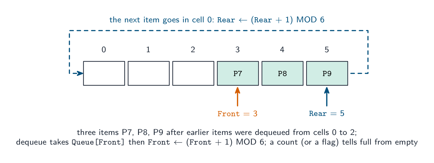
The Abstract Data Types (ADTs) from Topic 10 appear inside many algorithms: a stack 栈 drives depth-first traversal and undo; a queue 队列 drives breadth-first traversal and print ordering; a linked list 链表 lets data grow and shrink.
ADTs can be built from other ADTs, not just from arrays: a queue from two stacks; a stack from a linked list (push = prepend a head node 节点); a queue from a linked list with head and tail pointers 指针; a binary tree 二叉树 from nodes with two child pointers; a dictionary 字典 stores key→value pairs (often on a hash table). Layering this way separates concerns — the algorithm using the ADT need not know how it is built.
The ADTs the exam asks you to describe and implement
Stack (last in, first out): items are added (pushed) and removed (popped) at the same end, the top; a pointer TopOfStack holds the index of the top item. Implemented with an array and that one pointer: push checks the stack is not full, increments the pointer and stores the item; pop checks it is not empty, returns the top item and decrements the pointer.
FUNCTION Push(Item : INTEGER) RETURNS BOOLEAN
    IF TopOfStack = 9 THEN      // full (array 0 to 9)
        RETURN FALSE
    ENDIF
    TopOfStack ← TopOfStack + 1
    StackData[TopOfStack] ← Item
    RETURN TRUE
ENDFUNCTION
FUNCTION Pop() RETURNS INTEGER
    IF TopOfStack = -1 THEN      // empty
        RETURN -1
    ENDIF
    TopOfStack ← TopOfStack - 1
    RETURN StackData[TopOfStack + 1]
ENDFUNCTION
Queue (first in, first out): items join at the rear (enqueue) and leave from the front (dequeue); two pointers and a count. In a linear queue the front pointer creeps along the array until the space at the start is wasted; a circular queue 循环队列 wraps both pointers round with MOD, so every cell is reused.
FUNCTION Enqueue(Item : STRING) RETURNS BOOLEAN
    IF Count = 6 THEN      // full
        RETURN FALSE
    ENDIF
    Rear ← (Rear + 1) MOD 6
    QueueArray[Rear] ← Item
    Count ← Count + 1
    RETURN TRUE
ENDFUNCTION
FUNCTION Dequeue() RETURNS STRING
    IF Count = 0 THEN      // empty
        RETURN ""
    ENDIF
    DECLARE Item : STRING
    Item ← QueueArray[Front]
    Front ← (Front + 1) MOD 6
    Count ← Count - 1
    RETURN Item
ENDFUNCTION
Linked list: a sequence of nodes, each holding a data item and a pointer to the next node; a start pointer gives the first node and a null pointer (0 or $-1$) ends the list. In an array implementation two parallel arrays hold the data and the pointers, and unused cells are chained into a free list 空闲列表 so that an insertion knows where to put the new node.
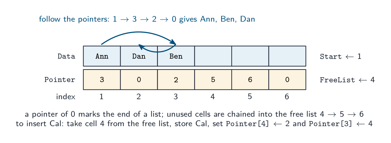
FUNCTION FindInList(Target : STRING) RETURNS INTEGER   // index, or 0 if absent
    DECLARE Current : INTEGER
    Current ← Start
    WHILE Current <> 0
        IF Data[Current] = Target THEN
            RETURN Current
        ENDIF
        Current ← Pointer[Current]
    ENDWHILE
    RETURN 0
ENDFUNCTION
To insert into an ordered list: take the first free cell (NewNode ← FreeList, FreeList ← Pointer[FreeList]), store the item, then walk the list with a Previous and Current pointer until Data[Current] > Item or the end; set Pointer[NewNode] ← Current and Pointer[Previous] ← NewNode (or Start ← NewNode if it goes first). To delete, re-link the previous node past the deleted one and return the cell to the free list.
Binary tree: a root node, each node holding data, a left pointer to a subtree of smaller values and a right pointer to a subtree of larger values. Implemented as a 2D array (or three 1D arrays) Tree[Index, 0..2] for left pointer, data, right pointer, with a root pointer and a next-free pointer.
FUNCTION FindInTree(Target : INTEGER) RETURNS INTEGER   // index, or -1
    DECLARE Current : INTEGER
    Current ← Root
    WHILE Current <> -1
        IF Tree[Current, 1] = Target THEN
            RETURN Current
        ENDIF
        IF Target < Tree[Current, 1] THEN
            Current ← Tree[Current, 0]      // go left
        ELSE
            Current ← Tree[Current, 2]      // go right
        ENDIF
    ENDWHILE
    RETURN -1
ENDFUNCTION
To insert: store the item in the next free node with both pointers $-1$; if the tree is empty make it the root; otherwise walk down from the root, going left or right by comparison, until the pointer you would follow is $-1$, and set that pointer to the new node. An ADT from another ADT: a stack is a linked list where push and pop both work at the start; a queue is a linked list with a start and an end pointer; a queue can be made from two stacks (push onto one, pop from the other, moving everything across when the second is empty); a binary tree's nodes are records or objects linked by pointers, so it is built from a linked structure of nodes. Say which operations of the new ADT map onto which operations of the old one.


Vocabulary
Train
| English |
|---|
| linked list/lɪŋkt lɪst/ |
| stack/stæk/ |
| queue/kjuː/ |
| node/nəʊd/ |
| pointers/ˈpɔɪntəz/ |
| binary tree/ˈbaɪnəri triː/ |
| dictionary/ˈdɪkʃənəri/ |
| circular queue/ˈsɜːkjʊlə kjuː/ |
| free list/friː lɪst/ |
19.1
Comparing algorithms
Time complexity
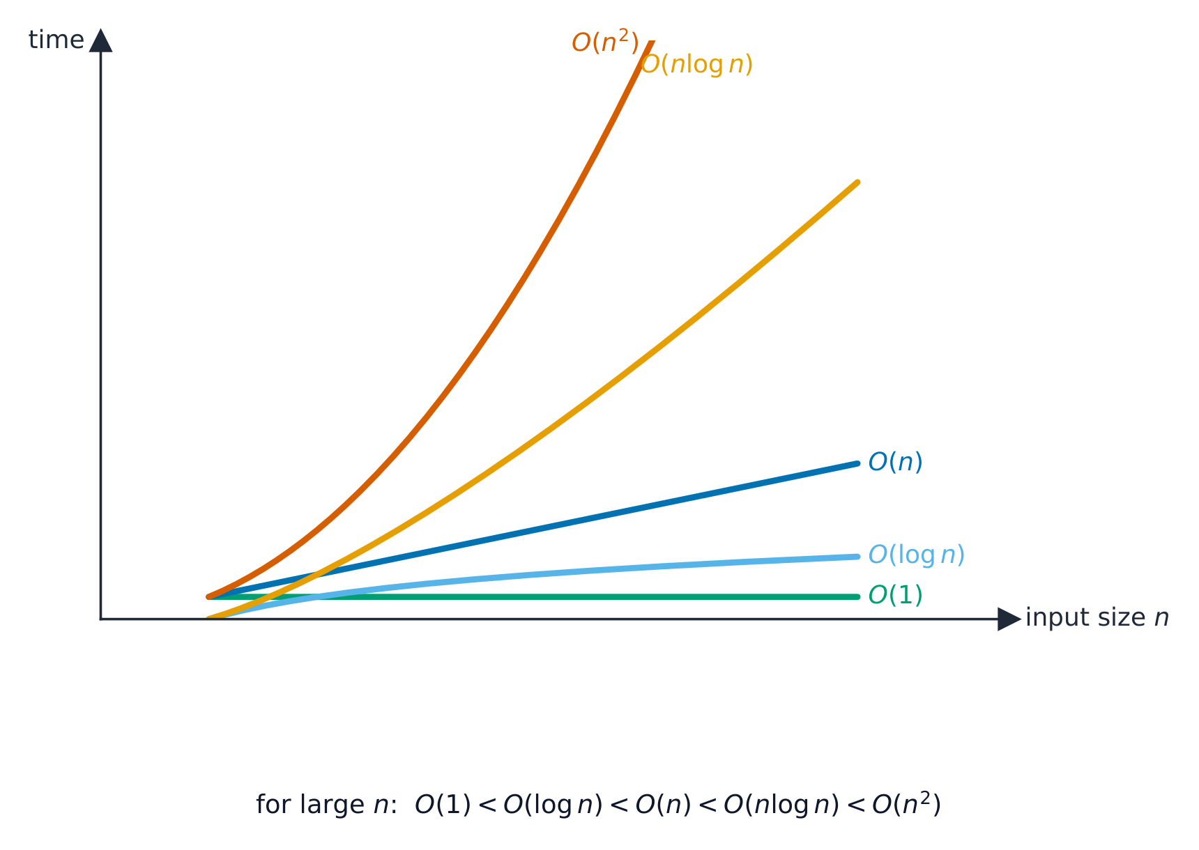
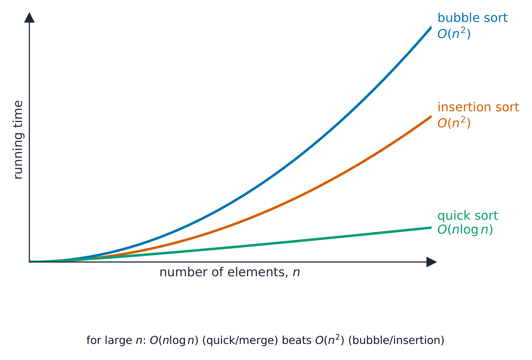
Time complexity 时间复杂度 is how the running time grows with input size $n$, written in Big-O notation 大O表示法 (the dominant term): O(1) constant, O($\log n$) binary search, O($n$) linear search, O($n \log n$) good sorts, O($n^{2}$) bubble/insertion sort. A smaller order is better at scale, even if another algorithm is faster for small $n$.
To make that concrete: to sort a million items, an $O(n \log n)$ sort finishes in a fraction of a second, while an $O(n^{2})$ sort can take minutes.
Worked example. A sorted list holds $1000$ items. How many comparisons does each search need in the worst case?
A linear search checks items one at a time, so it may need up to $1000$ comparisons — this is $O(n)$. A binary search halves the list each step, so it needs at most $\lceil \log_2 1000 \rceil = 10$ comparisons — this is $O(\log n)$. Doubling the list to $2000$ items adds only one comparison to the binary search, but up to another $1000$ to the linear search — which is why the order of growth, not raw speed, decides the winner at scale.
Describing an order. O(1): the time is constant, independent of the number of items (pushing onto a stack, reading an array element). O($\log n$): the time grows with the logarithm of the number of items, so doubling the data adds only a fixed extra step (binary search). O($n$): the time grows in proportion to the number of items (linear search, one pass through a list). O($n \log n$): a little worse than linear (efficient sorts). O($n^{2}$): the time grows with the square of the number of items, so doubling the data quadruples the time (bubble and insertion sort). "State the Big O of a binary search of Names[0:99]" is answered $O(\log n)$, and "describe its meaning" as above; Big O measures how the time or memory scales, not the actual time.
Space complexity
Space complexity 空间复杂度 is the extra memory needed. Bubble and insertion sort use O(1) extra (in place); merge sort uses O($n$); recursion uses stack memory proportional to its depth. There is often a time–memory trade-off.
Other criteria
Simplicity (easier to code and maintain), stability, and adaptiveness (faster on nearly-sorted data). The right algorithm depends on the data and the constraints.
Explore
How running time grows with n
Slide n upward and compare the curves: O(1) and O(log n) stay almost flat, O(n) rises steadily, O(n²) explodes. This is why Big-O — not a stopwatch — is how we compare algorithms on large inputs.
Explore
Big-O growth
Change the input size n and compare how fast each algorithm's work grows — the idea behind time complexity.
Vocabulary
Train
| English |
|---|
| time complexity/taɪm kəmˈpleksɪti/ |
| Big-O notation/bɪɡ əʊ nəʊˈteɪʃn/ |
| space complexity/speɪs kəmˈpleksɪti/ |
19.2
Recursion

Syllabus
| Candidates should be able to: | Notes and guidance |
|---|---|
| Show understanding of recursion | Essential features of recursion How recursion is expressed in a programming language Write and trace recursive algorithms When the use of recursion is beneficial |
| Show awareness of what a compiler has to do to translate recursive programming code | Use of stacks and unwinding |
Source: Cambridge International syllabus
Recursive algorithms use recursion 递归: the routine calls itself with a smaller version of the same problem, until a base case 基本情形 ends the chain. It has two parts: the base case (small enough to solve directly — without it the recursion never stops) and the recursive case 递归情形 (reduce the input and call itself).
Factorial 阶乘:
FUNCTION Factorial(n : INTEGER) RETURNS INTEGER
    IF n = 0 OR n = 1 THEN
        RETURN 1
    ELSE
        RETURN n * Factorial(n - 1)
    ENDIF
ENDFUNCTION
Recursion is natural for self-similar problems: trees, divide-and-conquer 分治 (binary search, merge sort), and nested data. When it is a poor fit, a loop is usually cleaner.
"Describe what is meant by recursion" (two marks). A function or procedure that is defined in terms of itself: it calls itself from within its own body, with a smaller version of the problem each time, until a base case is reached. "State three essential features of recursion": (1) a base case (stopping condition) that returns a value without a further call; (2) a general case 一般情形 in which the routine calls itself; (3) each call moves the problem closer to the base case (the parameter is reduced), so that the recursion terminates. Some schemes add: values are returned as the calls unwind.
"Describe when the use of recursion is beneficial, and give an example." When the problem is naturally defined in terms of smaller versions of itself, so that the recursive solution is shorter, clearer and closer to the mathematical definition than a loop would be: a factorial or Fibonacci number, a binary search, traversing a binary tree, merge sort or quicksort, and processing nested structures such as folders within folders. It is a poor choice when the depth is large (the stack may overflow) or when the same sub-problem is computed many times (naive Fibonacci).
Tracing a recursive call
For Factorial(4): the calls go down to Factorial(1)=1, then unwinding multiplies back up: 2*1=2, 3*2=6, 4*6=24. Final result 24. Track each pending call on a stack.
Worked example. The function below is given without an explanation. Trace Unknown(3, 5) and state its output and return value.
FUNCTION Unknown(BYVAL X, BYVAL Y : INTEGER) RETURNS INTEGER
    IF X < Y THEN
        OUTPUT X + Y
        RETURN Unknown(X + 1, Y - 1) + 1
    ELSE
        RETURN 0
    ENDIF
ENDFUNCTION
Call 1: $X = 3, Y = 5$: $3 < 5$, output 8, call Unknown(4, 4). Call 2: $4 < 4$ is false, return 0. Unwinding: call 1 returns $0 + 1 = 1$. Output 8, return value 1. Write the trace as a table with a row per call (parameters, condition, output, what it returns), and do the returns from the deepest call upwards: that is the unwinding the mark scheme looks for.
Worked example (Fibonacci). Fib(n) returns n when n < 2, otherwise Fib(n - 1) + Fib(n - 2). Find Fib(5).
Fib(5) = Fib(4) + Fib(3); Fib(4) = Fib(3) + Fib(2); Fib(3) = Fib(2) + Fib(1); Fib(2) = Fib(1) + Fib(0) = 1 + 0 = 1. So Fib(3) = 1 + 1 = 2, Fib(4) = 2 + 1 = 3, Fib(5) = 3 + 2 = 5. The base case is reached many times (Fib(2) is computed three times), which is why this version is slow: it makes 15 calls for $n = 5$ and roughly doubles the calls for every increase in $n$.
Converting recursion to iteration. Every recursive routine can be rewritten with a loop, which uses less memory and is faster: keep a running result and loop from the base case upwards. Factorial as a loop:
FUNCTION Factorial(N : INTEGER) RETURNS INTEGER
    DECLARE Result, Count : INTEGER
    Result ← 1
    FOR Count ← 2 TO N
        Result ← Result * Count
    NEXT Count
    RETURN Result
ENDFUNCTION
Asked to change a recursive insertion sort or search into an iterative one, replace the self-call with a loop over the index that the recursion was stepping through, and turn the base case into the loop's exit condition.
Risks
- infinite recursion if the base case is missed — crashes with a stack overflow 栈溢出.
- high memory use for deep recursion.
- slow if it repeats work (naive Fibonacci is exponential — use a loop or memoisation 记忆化).
Explore
Recursion unwinds from the leaves up
Step through fib(4) in the order the calls actually finish: the leaves (base cases) resolve first, then each parent combines its children. Notice fib(2) is computed twice — that repeated work is why naive recursion is slow.
Vocabulary
Train
| English |
|---|
| recursion/rɪˈkɜːʃn/ |
| base case/beɪs keɪs/ |
| recursive case/rɪˈkɜːsɪv keɪs/ |
| factorial/fækˈtɔːrɪəl/ |
| divide-and-conquer/dɪˈvaɪd ænd ˈkɒŋkə/ |
| general case/ˈdʒenərəl keɪs/ |
| stack overflow/stæk ˌəʊvəˈfləʊ/ |
| memoisation/ˌmeməʊaɪˈzeɪʃn/ |
19.2
What the compiler does for recursive code
Recursion needs each call to have its own copy of its parameters 参数 and local variables 局部变量. The compiler keeps these on the call stack 调用栈. For each call it pushes a stack frame 栈帧 holding the parameters, the local variables, and the return address 返回地址 (where to resume in the caller). When the function returns, the return value is handed back, the frame is popped, and control resumes at the return address.
Because each call has its own frame, recursive calls don't trample each other's variables. The stack can grow large for deep recursion, which is why very deep recursion may overflow it. This is the same call-and-return mechanism used for ordinary (non-recursive) calls — there is no special "recursion mechanism".
"Explain why a stack is suitable for implementing recursion" (three marks). Each recursive call must save its return address, its parameters and its local variables, and the calls are completed in the reverse order to that in which they were made (the last call made is the first to finish), which is exactly the last in, first out behaviour of a stack: each new call pushes a frame, and each return pops the most recent frame, restoring the caller's state and telling it where to continue. This is the compiler's job when it translates recursive code: it generates the push of a stack frame on every call and the pop on every return, and the frames are unwound as the results come back.
Vocabulary
Train
| English |
|---|
| call stack/kɔːl stæk/ |
| parameters/pəˈræmɪtəz/ |
| local variables/ˈləʊkl ˈveərɪəblz/ |
| stack frame/stæk freɪm/ |
| return address/rɪˈtɜːn əˈdres/ |
19.2
Definitions the examiner accepts
A definition question is marked against fixed wording. Learn these exactly, and give one answer only.
| Term | Definition |
|---|---|
| linear search | checking each item in turn from the start until the target is found or the end is reached |
| binary search | repeatedly comparing the target with the middle item of a sorted list and discarding the half that cannot contain it |
| bubble sort | repeatedly passing through the list, swapping adjacent items that are in the wrong order, until a pass makes no swaps |
| insertion sort | taking each item in turn and inserting it into its correct place among the items already sorted |
| abstract data type | a collection of data and the operations that can be performed on it, defined independently of how it is stored |
| stack | a last-in-first-out structure with push and pop at the top |
| queue | a first-in-first-out structure with items added at the rear and removed from the front |
| linked list | a sequence of nodes, each holding data and a pointer to the next node, with a start pointer |
| binary tree | nodes each holding data and pointers to a left subtree of smaller values and a right subtree of larger values |
| Big O notation | a way of classifying the time (or memory) an algorithm needs by how it grows with the size of the input |
| recursion | a routine that calls itself with a smaller version of the problem until a base case stops the calls |
| base case | the condition under which a recursive routine returns without calling itself |
| unwinding | the returns of a chain of recursive calls, from the deepest call back to the first, as the stack frames are popped |
19.2
Exam tips
- Searches: linear needs no order and O($n$); binary needs a sorted array, halves each time and is O($\log n$). Know both algorithms by heart, including the bounds and the flag.
- Sorts: bubble with a swapped flag, insertion with a key that shifts larger items right; both O($n^{2}$) worst, O($n$) on sorted data. Performance depends on the number of items and how ordered they are.
- ADT implementations are pointer bookkeeping: a top pointer; front, rear and count with MOD; start, pointers and a free list; root with left and right pointers. Always check for full and empty.
- Big O is about scaling: constant, logarithmic, linear, square. Say "doubling the data adds one comparison" for a binary search.
- Recursion: base case, general case, progress towards the base case; beneficial when the problem is defined in terms of itself; a stack holds the return addresses and variables because calls return in reverse order. Trace with a table and unwind from the deepest call.
Common mistakes
- Using a binary search on unsorted data, or on a linked list; and setting
Lower ← Midinstead ofMid + 1, which loops for ever. - A bubble sort inner loop that runs to the end of the array every pass, or a swap without a temporary variable.
- A push or enqueue that does not test for full, or a pop or dequeue that does not test for empty.
- Moving the queue's front pointer without MOD in a circular queue, or treating front = rear as always meaning empty.
- Inserting into a linked list by shifting the array contents; only the pointers change.
- A recursive function with no base case, or one whose recursive call does not make the problem smaller.
- Tracing a recursive call but forgetting to add the pending work on the way back up.
- Answering "why a stack" with "because it is fast"; the reason is the last-in-first-out order of the returns.
Interactive lessons on this topic
Work through it step by step, with instant-check exercises.