Edexcel IAL Fisika Unit 1 (paper WPH11) adalah Mekanika dan Material: bagaimana benda bergerak, apa yang dilakukan oleh gaya, bagaimana momentum dan energi berperilaku, serta bagaimana material padat dan cair merespons gaya.
Paper ini berdurasi 1 jam 30 menit, 80 skor, setiap soal wajib dijawab. Soal ini menggabungkan pilihan ganda, jawaban singkat, perhitungan, dan satu atau dua jawaban tulisan panjang yang ditandai dengan asterisk (*).
Minimal 32 dari 80 skor menguji matematika Level-2: membaca grafik, menyusun ulang persamaan, trigonometri, dan luas.
Daftar rumus dicetak di bagian belakang paper. Pelajari arti setiap simbol dan kapan setiap persamaan diperbolehkan — daftar tersebut memberikan rumus, bukan pemahaman.
Gunakan $g = 9.81\ \text{m s}^{-2}$. Paper memerlukan nilai ini; menggunakan $g = 10$ dapat menghilangkan poin akurasi. Berikan jawaban akhir dengan satuan dan jumlah angka penting yang masuk akal (biasanya 2–3, sesuai data).
Speedometer menunjukkan kecepatan pada satu momen; sebuah perjalanan bisa saja menyembunyikan berhenti dan percepatan mendadak. Unit ini menggantikan satu angka dengan gambaran utuh: grafik, vektor, gaya, momentum, energi, dan kekuatan material.
Mechanics and Materials/mɪˈkænɪks ænd məˈtɪərɪəlz/
Mekanika dan Material
asterisk/ˈæstərɪsk/
tanda bintang
trigonometry/ˌtrɪɡəˈnɒmətri/
trigonometri
unit/ˈjuːnɪt/
satuan
significant figures/sɪɡˈnɪfɪkənt ˈfɪɡəz/
angka penting
vectors/ˈvektəz/
vektor
forces/ˈfɔːsɪz/
gaya
momentum/məʊˈmentəm/
Momentum
speed/spiːd/
kecepatan
acceleration/əkˌseləˈreɪʃn/
percepatan
gradient/ˈɡreɪdɪənt/
gradien
tangent/ˈtændʒənt/
garis singgung
1.1
Gerak: besaran dan grafik
Silabus
Edexcel IAL Physics Unit 1 (WPH11), specification Issue 3 (July 2021), statements 1–3 and 11 (core practical 1; numbered between the force statements in the specification, taught here with motion).
be able to use the equations for uniformly accelerated motion in one dimension: s = (u+v)t/2, v = u + at, s = ut + ½at², v² = u² + 2as
be able to draw and interpret displacement–time, velocity–time and acceleration–time graphs
know the physical quantities derived from the slopes and areas of displacement–time, velocity–time and acceleration–time graphs, including cases of non-uniform acceleration, and understand how to use the quantities
CORE PRACTICAL 1: Determine the acceleration of a freely-falling object
Sumber: Silabus Cambridge International
perpindahan — perubahan posisi lurus dengan arah (vektor). jarak — total panjang lintasan (besaran skalar, tanpa arah).
kecepatan — laju perubahan perpindahan. kelajuan — laju perubahan jarak.
percepatan — laju perubahan kecepatan: $a = \dfrac{\Delta v}{\Delta t}$, satuan $\text{m s}^{-2}$.
Karena perpindahan adalah garis lurus dari awal ke akhir, lintasan melengkung selalu menghasilkan jarak > magnitudo perpindahan — penguji meminta perbandingan persis seperti ini.
Membaca grafik gerak
Pada grafik perpindahan–waktu, gradien adalah kecepatan. Garis lengkung berarti kecepatan berubah; ambil gradien dari garis singgung pada titik tersebut.
Pada grafik kecepatan–waktu, gradien adalah percepatan, dan luas antara garis dan sumbu waktu adalah perpindahan. Luas di bawah sumbu adalah perpindahan negatif (gerak mundur); jarak menjumlahkan ukuran semua luas.
Pada grafik percepatan–waktu, luas di bawah garis adalah perubahan kecepatan.
Percepatan konstan tak nol membengkokkan grafik perpindahan–waktu menjadi parabola; garis lurus pada grafik itu berarti percepatan nol.
Contoh terpecahkan (gaya Juni 2025). Garis kecepatan–waktu naik lurus dari $1.8\ \text{m s}^{-1}$ pada $t = 4\ \text{s}$ ke $5.0\ \text{m s}^{-1}$ pada $t = 16\ \text{s}$.
Diketahui: dua pasangan $(t, v)$ pada bagian lurus. Mengapa: percepatan adalah gradien dari grafik kecepatan–waktu.
Cek: garis naik landai, sehingga percepatan kecil masuk akal.
Empat persamaan suvat
Untuk percepatan seragam (percepatan konstan) dalam satu dimensi, dengan $s$ perpindahan, $u$ kecepatan awal, $v$ kecepatan akhir, $a$ percepatan, $t$ waktu:
$$v = u + at \qquad s = \frac{(u+v)t}{2} \qquad s = ut + \tfrac{1}{2}at^2 \qquad v^2 = u^2 + 2as$$
Pilih persamaan yang memuat besaran yang diketahui dan yang ingin dicari—dan tidak ada yang tidak diketahui. Tidak ada $t$? Gunakan $v^2 = u^2 + 2as$. Tidak ada $a$? Gunakan $s = \tfrac{(u+v)}{2}t$.
Persamaan-persamaan ini hanya berlaku selama percepatan konstan. Grafik kecepatan–waktu yang melengkung menunjukkan percepatan berubah; grafik perpindahan–waktu yang melengkung masih bisa mewakili percepatan konstan.
Jatuh bebas adalah percepatan seragam dengan $a = g = 9.81\ \text{m s}^{-2}$ ke bawah (gaya hambat udara diabaikan).
Contoh terpecahkan (deduksi-dan-bandingkan, Juni 2025 Q13). Sebuah bola basket dilempar dari ketinggian $1.7\ \text{m}$ di atas lantai dengan kecepatan vertikal awal $5.1\ \text{m s}^{-1}$ ke atas, dan masuk ke ring bergerak ke bawah pada kecepatan $2.1\ \text{m s}^{-1}$. Apakah ring berada pada ketinggian $3.0\ \text{m}$ di atas lantai?
Diketahui: $u = +5.1\ \text{m s}^{-1}$, $v = -2.1\ \text{m s}^{-1}$ (ke bawah bernilai negatif), $a = -9.81\ \text{m s}^{-2}$. Ditanyakan: kenaikan $\Delta s$. Tidak ada waktu yang diberikan, jadi gunakan $v^2 = u^2 + 2a\Delta s$.
$$v^2 = u^2 + 2a\Delta s \quad\Rightarrow\quad \Delta s = \frac{v^2 - u^2}{2a}$$
Tinggi ring $= 1.7\ \text{m} + 1.1\ \text{m} = 2.8\ \text{m} \neq 3.0\ \text{m}$, sehingga ring tersebut tidak berada pada ketinggian standar. Soal "tentukan apakah" mendapatkan nilai penuh hanya jika perbandingan dan kesimpulan dinyatakan secara eksplisit.
Praktikum inti 1: mengukur $g$
Jatuhkan sebuah benda dan ukur: dengan gerbang cahaya atau video dengan laju bingkai yang diketahui, peroleh $s$ dan $t$ (atau kecepatan di dua titik) lalu gunakan persamaan suvat. Lebih baik: plot $s$ terhadap $t^2$ untuk $s = \tfrac{1}{2}gt^2$ — garis lurus melalui titik asal dengan gradien $g/2$. Garis lurus yang tidak melewati titik asal mengindikasikan adanya offset sistematis, misalnya offset tetap pada jarak terukur. Keterlambatan pengatur waktu juga dapat mendistorsi hubungan; pengatur waktu otomatis mengurangi kesalahan reaksi. Dalam foto strobo, benda bergerak selama setiap kilatan flash. Flash yang lebih pendek menghasilkan gambar yang lebih tajam dan rentang posisi yang lebih kecil, mengurangi ketidakpastian pembacaan jarak jika skala dan resolusi gambar tetap.
memahami besaran skalar dan vektor serta mengetahui contoh masing-masing jenis besaran dan mengenali notasi vektor
mampu menguraikan sebuah vektor menjadi dua komponen yang saling tegak lurus dengan cara menggambar dan perhitungan
mampu menemukan resultan dua vektor sebidang pada sudut apa pun terhadapnya dengan menggambar, dan pada sudut tegak lurus terhadapnya dengan perhitungan
memahami cara memanfaatkan independensi gerak vertikal dan horizontal proyektil yang bergerak bebas di bawah gravitasi
Sumber: Silabus Cambridge International
Sebuah vektor memiliki besar dan arah (perpindahan, kecepatan, percepatan, gaya, momentum); skalar hanya memiliki besar (jarak, kelajuan, usaha, energi). Notasi vektor dalam soal ditunjukkan dengan panah di atas simbol, $\vec{F}$.
Menguraikan dan menggabungkan
Menguraikan memecah satu vektor menjadi dua komponen saling tegak lurus: komponen gaya $F$ pada sudut $\theta$ sepanjang suatu arah adalah $F\cos\theta$ jika $\theta$ diukur dari arah tersebut, $F\sin\theta$ dari arah tegak lurusnya. Tentukan dengan menggambar segitiga siku-siku, bukan berdasarkan kebiasaan.
Menggabungkan dua komponen saling tegak lurus membangun kembali vektor: besar $R = \sqrt{F_x^2 + F_y^2}$, arah ditentukan oleh $\tan\theta = F_y / F_x$.
Gabungkan sebelum dikuadratkan. Resultan dari $500\ \text{N}$ dan $200\ \text{N}$ yang saling tegak lurus adalah $\sqrt{500^2 + 200^2}\ \text{N}$, bukan $\sqrt{500^2} + \sqrt{200^2}$.
Pada sudut berapa pun, tambahkan vektor dengan menggambar diagram skala (segitiga vektor, ujung ke ekor) atau dengan menguraikan masing-masing vektor menjadi komponen terlebih dahulu. Dalam kesetimbangan, segitiga vektor tertutup: $\vec{W} + \vec{T_1} + \vec{T_2} = 0$.
Contoh terpecahkan. Sebuah kotak berada di bidang miring dengan sudut $\theta$ terhadap horizontal, beratnya $W$ bekerja tegak lurus ke bawah.
Mengapa: arah seluncur sejajar dengan bidang miring, jadi uraikan $W$ menjadi komponen sejajar dan tegak lurus terhadap bidang miring.
Pada kecepatan konstan, resultan gaya adalah nol, sehingga gesekan $F = W\sin\theta$ secara tepat. ($W\cos\theta$ bekerja ke dalam bidang miring dan diimbangi oleh gaya kontak normal.)
Gerak peluru
Peluru yang bergerak bebas di bawah gravitasi mengalami dua gerak independen: kecepatan horizontal konstan (tidak ada gaya horizontal), kecepatan vertikal berubah akibat $g$.
Waktu jatuh hanya bergantung pada gerak vertikal. Dua bola yang meninggalkan meja dengan kecepatan berbeda — atau massa berbeda — mendarat setelah waktu yang sama: massa dan kecepatan horizontal tidak muncul dalam $s = ut + \tfrac{1}{2}gt^2$.
Metode: uraikan kecepatan awal menjadi komponen $u_h = u\cos\theta$ dan $u_v = u\sin\theta$; terapkan persamaan suvat secara terpisah untuk setiap arah; waktu menghubungkan keduanya.
Contoh terpecahkan (Januari 2025 Q19). Sebuah peluru diluncurkan dengan $500\ \text{m s}^{-1}$, $22^\circ$ di atas garis horizontal, dari ketinggian $2.0\ \text{km}$ di atas permukaan laut. Tunjukkan bahwa peluru tersebut melewati kapal yang berjarak $15\ \text{km}$ setelah sekitar $30\ \text{s}$.
Diketahui: $u$, $\theta$, jarak horizontal $s_h$. Gerak horizontal memiliki $a = 0$, sehingga gunakan $s_h = u_h t$.
Mengapa terdapat jangkauan maksimum: meningkatkan sudut peluncuran meningkatkan $u_v$ (waktu lebih lama di udara) tetapi menurunkan $u_h$; jangkauan $= u_h \times t$ mencapai puncaknya di antara kedua efek tersebut.
gravitational field strength/ˌɡrævɪˈteɪʃənl fiːld streŋθ/
kekuatan medan gravitasi
terminal velocity/ˈtɜːmɪnl vəˈlɒsɪti/
kecepatan terminal
drag/dræɡ/
hambatan
conservation of linear momentum/ˌkɒnsəˈveɪʃn ɒv ˈlɪnɪə məʊˈmentəm/
kekekalan momentum linear
isolated system/ˈaɪsəleɪtɪd ˈsɪstəm/
sistem terisolasi
moment of a force/ˈməʊmənt əvə fɔːs/
torsi gaya
1.3
Gaya dan Hukum Newton
Silabus
Edexcel IAL Fisika Unit 1 (WPH11), spesifikasi Edisi 3 (Juli 2021), pernyataan 8–10 dan 12 (pernyataan 11, praktik inti 1, diajarkan pada lembar 1.1 dengan gerak).
mampu menggambar dan menafsirkan diagram gaya bebas untuk merepresentasikan gaya yang bekerja pada partikel atau pada benda terluas namun kaku menggunakan konsep pusat gravitasi benda terluas
mampu menggunakan persamaan ΣF = ma, dan memahami cara menggunakan persamaan ini dalam situasi di mana m konstan (hukum kedua Newton tentang gerak), termasuk hukum pertama Newton tentang gerak di mana a = 0, benda diam atau bergerak dengan kecepatan konstan; penggunaan istilah kecepatan terminal diharapkan
mampu menggunakan persamaan untuk kekuatan medan gravitasi g = F/m dan berat W = mg
mengetahui dan memahami hukum ketiga Newton tentang gerak serta mengetahui sifat pasangan gaya dalam interaksi antara dua benda
Sumber: Silabus Cambridge International
Diagram benda bebas hanya menunjukkan gaya-gaya yang bekerja pada objek yang dipilih — bukan gaya yang objek terapkan pada benda lain. Pada benda memanjang, berat bekerja pada pusat gravitasi.
Hukum pertama Newton: resultan gaya nol berarti tidak ada perubahan gerak — diam atau bergerak dengan kecepatan konstan. Kecepatan konstan bukan "tanpa gaya"; melainkan gaya-gaya yang seimbang.
Hukum kedua Newton: $\sum F = ma$. Resultan gaya menyebabkan percepatan; daftar semua gaya, pilih arah positif, lalu terapkan.
Hukum ketiga Newton: ketika tubuh A menerapkan gaya pada tubuh B, B menerapkan gaya yang sama besar dan berlawanan arah pada A. Pasangan ini bekerja pada tubuh yang berbeda, merupakan jenis gaya yang sama, dan bekerja sepanjang garis lurus. Berat buku dan gaya kontak normal meja bukan pasangan hukum ketiga: keduanya bekerja pada tubuh yang sama.
berat$W = mg$; keku medan gravitasi$g = \dfrac{F}{m}$, sehingga $g = 9.81\ \text{N kg}^{-1}$.
Kecepatan terminal: saat benda jatuh semakin cepat, gaya hambat meningkat hingga gaya hambat (+ gaya apung) sama dengan berat; resultan gaya kemudian menjadi nol dan kecepatan berhenti berubah. "Terminal" menggambarkan keseimbangan gaya, bukan batas kecepatan yang tertulis dalam alam.
Contoh terpecahkan (Juni 2025 Q11). Resultan gaya sebesar $4800\ \text{N}$ memberikan percepatan pada perahu sebesar $0.31\ \text{m s}^{-2}$. Temukan berat perahu.
Diketahui: $\sum F$, $a$. Alasan: $\sum F = ma$ menghubungkannya dengan massa; $W = mg$ menghubungkan massa dengan berat.
$$\sum F = ma \quad\Rightarrow\quad m = \frac{\sum F}{a} = \frac{4800\ \text{N}}{0.31\ \text{m s}^{-2}} = 15\,500\ \text{kg}$$
memahami bahwa momentum didefinisikan sebagai p = mv
mengetahui prinsip kekekalan momentum linear, memahami bagaimana menghubungkannya dengan hukum-hukum Newton tentang gerak dan memahami bagaimana menerapkannya pada masalah dalam satu dimensi
Sumber: Silabus Cambridge International
momentum$p = mv$, besaran vektor, satuan $\text{kg m s}^{-1}$.
Hukum Kekekalan Momentum Linear: ketika resultan gaya eksternal nol (atau impulsnya dapat diabaikan selama interaksi singkat), total momentum sebelum peristiwa sama dengan total momentum setelahnya. Berikan tanda pada kecepatan: pilih satu arah sebagai positif dan pertahankan itu.
Kekekalan momentum diturunkan dari Hukum Kedua dan Ketiga Newton: gaya antara dua benda besarnya sama dan berlawanan arah, bekerja selama waktu yang sama, sehingga perubahan momentumnya juga sama besar dan berlawanan arah.
Energi kinetik tidak harus bertahan dalam tumbukan; momentum selalu kekal (dalam sistem terisolasi).
Contoh Kerja (Juni 2025 Q10). Kereta bermassa $3m$ bergerak dengan kecepatan $v$ menabrak truk bermassa $m$ bergerak ke arah berlawanan dengan kecepatan $2v$; keduanya tersambung. Tentukan kecepatan baru tersebut.
Diketahui: massa dan kecepatan berlawanan arah. Mengapa: pasangan terisolasi, sehingga gunakan kekekalan momentum dengan tanda. Arah kereta diambil sebagai positif.
$$p_{\text{before}} = p_{\text{after}}$$
$$3m \times v + m \times (-2v) = (3m + m)\,V$$
$$mv = 4mV \quad\Rightarrow\quad V = \frac{v}{4}$$
Cek: momentum hampir saling menghilangkan, sehingga kecepatan gabungan yang kecil searah kereta adalah masuk akal.
mampu menggunakan persamaan momen gaya, momen gaya = Fx, di mana x adalah jarak tegak lurus antara garis kerja gaya dan sumbu rotasi
mampu menggunakan konsep pusat gravitasi benda terluas dan menerapkan prinsip momen pada benda terluas dalam keadaan setimbang
Sumber: Silabus Cambridge International
Momen gaya terhadap titik tumpu adalah $\text{moment} = Fx$, di mana $x$ adalah jarak tegak lurus dari titik tumpu ke garis kerja gaya. Jika gaya memotong tuas pada sudut $\theta$, gunakan komponen tegak lurus $F\sin\theta$ atau jarak tegak lurus — jangan keduanya.
Prinsip Momen: dalam kesetimbangan, total momen searah jarum jam = total momen berlawanan arah jarum jam (resultan momen nol).
Kesetimbangan penuh memerlukan keduanya: resultan gaya nol dan resultan momen nol. Ayunan anak dengan berat sama pada jarak sama memiliki keduanya; berat yang sama namun jarak berbeda tetap menyeimbangkan gaya tetapi bukan momen.
Untuk balok seragam, beratnya bekerja pada pusatnya.
Contoh Kerja (Juni 2025 Q19.) Rel seragam, panjang $1.40\ \text{m}$, berat $95\ \text{N}$, terletak miring $42^\circ$ terhadap horizontal, dipivotkan di salah satu ujungnya. Piston mendorong dengan gaya $160\ \text{N}$ pada sudut $18^\circ$ terhadap rel, sejauh $0.37\ \text{m}$ dari pivot. Berapa besar gaya tegak lurus $F$ di ujung pegangan yang tepat mengangkat rel?
Diketahui: geometri, kedua gaya, kedua sudut. Mengapa: tepat saat diangkat berarti kesetimbangan di pivot, jadi terapkan prinsip momen dengan komponen tegak lurusnya.
Tarikan vertikal di pegangan: jarak tegak lurusnya ke pivot lebih pendek dari panjang rel, sehingga gaya yang lebih besar diperlukan untuk menghasilkan momen yang sama.
mampu menggunakan persamaan untuk usaha ΔW = FΔs, termasuk perhitungan ketika gaya tidak sepanjang garis gerak
mampu menggunakan persamaan Ek = ½mv² untuk energi kinetik suatu benda
mampu menggunakan persamaan ΔEgrav = mgΔh untuk perbedaan energi potensial gravitasi dekat permukaan Bumi
mengetahui dan memahami bagaimana menerapkan prinsip kekekalan energi termasuk penggunaan usaha, energi potensial gravitasi, dan energi kinetik
mampu menggunakan persamaan yang menghubungkan daya, masa dan tenaga yang dipindahkan atau usaha yang dilakukan P = E/t dan P = W/t
mampu menggunakan persamaan kecekapan = tenaga berguna keluar / total tenaga masuk dan kecekapan = daya berguna keluar / total daya masuk
Sumber: Silabus Cambridge International
usaha$\Delta W = F\Delta s$ ketika gaya bekerja sepanjang gerak; jika gaya membentuk sudut $\theta$ terhadap gerak, hanya komponen sejajar gerak yang melakukan usaha: $\Delta W = F\Delta s\cos\theta$.
energi kinetik$E_k = \tfrac{1}{2}mv^2$ — menggandakan kecepatan mengalikan empat kali energinya.
energi potensial gravitasi$\Delta E_{\text{grav}} = mg\Delta h$ di dekat permukaan Bumi.
Hukum kekekalan energi: energi ditransfer atau diubah, tidak pernah diciptakan atau dimusnahkan. Dalam jatuh dengan hambatan udara, $\Delta E_{\text{grav}}$ berubah menjadi $E_k$ditambah usaha yang dilakukan melawan hambatan udara; pada kecepatan terminal $E_k$ konstan, sehingga seluruh$\Delta E_{\text{grav}}$ dialokasikan untuk usaha melawan hambatan.
daya$P = \dfrac{E}{t} = \dfrac{W}{t}$ — energi yang ditransfer per satuan waktu.
efisiensi$= \dfrac{\text{useful energy output}}{\text{total energy input}} = \dfrac{\text{useful power output}}{\text{total power input}}$.
Contoh terpecah (Juni 2025 Q14). Mobil listrik bermassa $1800\ \text{kg}$ bergerak dengan kecepatan $14\ \text{m s}^{-1}$ lalu direm hingga berhenti di atas bukit, mendapatkan ketinggian $0.76\ \text{m}$; baterai mengakumulasi energi $45\ \text{kJ}$. Hitung efisiensi pengereman tersebut.
Diketahui: $m$, $v$, $\Delta h$, penambahan energi baterai. Mengapa: total input adalah energi yang diambil oleh rem — yaitu energi kinetik yang hilang dikurangi energi potensial gravitasi yang tetap dimiliki mobil karena berakhir pada posisi lebih tinggi.
understand how to use the relationship upthrust = weight of fluid displaced
a) be able to use the equation for viscous drag (Stokes' law) F = 6πηrv; b) understand that this equation applies only to small spherical objects moving at low speeds with laminar flow (or in the absence of turbulent flow) and that viscosity is temperature dependent
CORE PRACTICAL 2: Use a falling-ball method to determine the viscosity of a liquid
Sumber: Silabus Cambridge International
kerapatan$\rho = \dfrac{m}{V}$. Untuk bola, $V = \tfrac{4}{3}\pi r^3$.
gaya apung = berat fluida yang dipindahkan — yaitu berat fluida yang dipindahkan, bukan volume atau massanya.
Hukum Stokes: hambatan viskos pada bola kecil berkecepatan rendah dalam aliran laminar adalah $F = 6\pi\eta rv$, dengan $\eta$ sebagai kekentalan, $r$ sebagai jari-jari, dan $v$ sebagai kecepatan. Hukum ini hanya berlaku untuk bola kecil yang bergerak lambat tanpa turbulensi, dan $\eta$ menurun ketika cairan memanas dalam eksperimen ini; gas umumnya tidak mengikuti tren ini.
Praktikum inti 2: mengukur kekentalan dengan metode bola jatuh
Jatuhkan bola bantalan ke dalam tabung ukur berisi cairan. Tunggu hingga bola jatuh dengan kecepatan terminal, kemudian catat waktu tempuhnya pada jarak yang telah ditandai. Pada kecepatan terminal, gaya-gaya seimbang: berat = gaya apung + hambatan, sehingga
Anda memerlukan jari-jari dan massa bola (atau kerapatannya), kerapatan minyak, jarak jatuh, dan waktu. Minyak hangat memiliki kekentalan lebih rendah, sehingga bola jatuh lebih cepat dan waktu yang diukur menjadi lebih singkat.
be able to use the Hooke's law equation ΔF = kΔx, where k is the stiffness of the object
understand how to use the relationships (tensile or compressive) stress = force / cross-sectional area, (tensile or compressive) strain = change in length / original length, and Young modulus = stress / strain
a) be able to draw and interpret force–extension and force–compression graphs; b) understand the terms limit of proportionality, elastic limit, yield point, elastic deformation and plastic deformation and be able to apply them to these graphs
be able to draw and interpret tensile or compressive stress–strain graphs, and understand the term breaking stress
CORE PRACTICAL 3: Determine the Young modulus of a material
be able to calculate the elastic strain energy Eel in a deformed material sample, using the equation ΔEel = ½FΔx, and from the area under the force–extension graph; the estimation of area and hence energy change for both linear and non-linear force–extension graphs is expected
Sumber: Silabus Cambridge International
Hukum Hooke: $\Delta F = k\,\Delta x$ selama material berperilaku secara proporsional; $k$ adalah kekakuan (konstanta pegas), yaitu kemiringan grafik gaya–regangan.
tegangan$\sigma = \dfrac{F}{A}$ (satuan Pa), regangan$\varepsilon = \dfrac{\Delta x}{x}$ (tanpa satuan), modulus Young$E = \dfrac{\sigma}{\varepsilon}$. Tegangan dan regangan mendeskripsikan material; gaya dan pertambahan panjang mendeskripsikan sampel.
Pada grafik gaya–regangan atau tegangan–regangan: bagian lurus berakhir pada batas proporsional; melewati batas elastis, sampel tidak kembali ke panjang aslinya (deformasi elastis = kembali; deformasi plastis = tetap meregang); material dengan titik leleh yang jelas dapat meregang signifikan dengan sedikit peningkatan gaya saat titik leleh; material ulet lainnya mengalami leleh secara bertahap. Titik leleh menandai awal aliran plastis yang signifikan; tegangan putus adalah tegangan saat patah.
energi regangan elastis: $\Delta E_{\text{el}} = \tfrac{1}{2}F\Delta x$ untuk pegas linear — yaitu area di bawah grafik gaya–regangan. Untuk grafik non-linear, estimasi area menggunakan kotak-kotak. Area di bawah grafik tegangan–regangan pemuatan adalah usaha yang dilakukan per satuan volume, karena $\dfrac{F}{A} \times \dfrac{\Delta x}{x} = \dfrac{F\Delta x}{V}$. Di daerah elastis, energi ini tersimpan secara reversibel sebagai energi regangan elastis; usaha melebihi batas elastis tidak semuanya dapat dikembalikan.
Contoh terpecah (Juni 2025 Q17b). Senar biola dengan panjang asli $0.750\ \text{m}$ dan jari-jari $0.85 \times 10^{-3}\ \text{m}$ meregang sejauh $0.752\ \text{m}$ di bawah gaya $36\ \text{N}$. Hitung modulus Young-nya.
Diketahui: $F$, $x$, $\Delta x$, $r$. Mengapa: $E = \sigma/\varepsilon$ memerlukan tegangan dan regangan; tegangan memerlukan luas penampang.
Cek: modulus kawat logam adalah $10^{9}$–$10^{12}\ \text{Pa}$; $6\ \text{GPa}$ berada dalam rentang tersebut.
Praktikum inti 3: modulus Young pada kawat
Gantungkan beban yang diketahui pada kawat panjang dan ukur pertambahan panjang dengan penanda di samping penggaris; jaga agar kawat panjang dan pertambahan kecil untuk presisi, tambahkan beban secara bertahap dalam daerah proporsional, dan ukur diameter di beberapa tempat dengan mikrometer sekrup. Kemudian $E$ diperoleh dari kemiringan garis tegangan–regangan, atau dari $\sigma/\varepsilon$ titik per titik dalam daerah proporsional.
limit of proportionality/ˈlɪmɪt ɒv prəˌpɔːʃəˈnælɪti/
batas proporsionalitas
elastic limit/ɪˈlæstɪk ˈlɪmɪt/
batas elastis
elastic deformation/ɪˈlæstɪk ˌdiːfɔːˈmeɪʃn/
deformasi elastis
plastic deformation/ˈplæstɪk ˌdiːfɔːˈmeɪʃn/
deformasi plastis
yield point/jiːld pɔɪnt/
titik leleh
breaking stress/ˈbreɪkɪŋ stres/
tegangan patah
elastic strain energy/ɪˈlæstɪk streɪn ˈenədʒi/
energi regangan elastis
per unit volume/pɜː ˈjuːnɪt ˈvɒljuːm/
per satuan volume
micrometer/maɪˈkrɒmɪtə/
mikrometer sekrup
1.8
Kiat ujian untuk WPH11
Tunjukkan setiap langkah. "Penggunaan $F = ma$" mendapat nilai sebelum angka muncul — tuliskan persamaan dalam simbol, lalu substitusikan.
Satuan dan $g$. Ketidakjelasan satuan biasanya menyebabkan hilangnya nilai akhir; $g = 10\ \text{m s}^{-2}$ dapat mengurangi akurasi; soal "buktikan" membutuhkan satu angka penting lebih banyak daripada nilai target.
Kata perintah:nyatakan = jawaban singkat dan tepat; hitung/tentukan = angka beserta perhitungan dan satuan; turunkan = perhitungan plus kesimpulan dibandingkan; jelaskan = alasan fisika yang saling terkait; deskripsikan = apa yang terjadi, berurutan.
Jawaban bintang (*) dinilai berdasarkan penalaran logis yang terhubung serta konten: urutkan poin-poinnya, lalu hubungkan.
Daftar rumus ada di bagian belakang — ketahui lokasinya, sehingga Anda tidak perlu menghafal hal yang bisa dilihat dalam dua detik.
1.8
Periksa diri Anda
Pada grafik kecepatan–waktu, apa yang ditunjukkan oleh kemiringan dan luas area? — percepatan; perpindahan.
Persamaan suvat manakah yang mencari ketinggian dari dua kecepatan tanpa waktu? — $v^2 = u^2 + 2as$.
Percepatan horizontal peluru dalam penerbangan bebas? — nol (hanya gravitasi yang bekerja, vertikal).
Sebuah buku diam di atas meja: apakah beratnya dan gaya normal meja merupakan pasangan hukum ketiga Newton? — Tidak: keduanya bekerja pada benda yang sama.
Dua troli bertabrakan dan menyatu. Besaran mana yang selalu kekal? — total momentum (energi kinetik tidak harus kekal).
Gaya miring terhadap tuas: jarak mana yang masuk ke dalam momen? — jarak tegak lurus dari poros ke garis kerja gaya.
Mobil mengerem menanjak: apa energi input untuk efisiensi? — energi kinetik yang hilang dikurangi energi potensial gravitasi yang didapat.
Gaya apung setara dengan berat apa? — fluida yang dipindahkan.
Hukum Stokes memerlukan tiga kondisi apa? — bola kecil, kecepatan rendah, aliran laminar (dan $\eta$ bergantung suhu).
Pada grafik tegangan–regangan, apa kemiringan bagian lurus dan luas di bawahnya? — modulus Young; energi regangan elastis per satuan volume.
Pearson Edexcel IAL Physics, WPH12/01, Issue 3 (July 2021), printed pp.20–23 (PDF pp.24–27).
Main-loop faithful transcription of numbered requirements; mathematical text normalised from the PDF text layer. This is syllabus scope, not a student handout.
Understand amplitude, frequency, period, speed and wavelength.
Use the wave equation v = fλ.
Describe longitudinal waves in terms of pressure variation and displacement of molecules.
Describe transverse waves.
Draw and interpret graphs representing transverse and longitudinal waves, including standing/stationary waves.
Sumber: Silabus Cambridge International
2.2Superposition and standing waves (statements 38–43, core practicals 4–5)
Pearson Edexcel IAL Physics, WPH12/01, Issue 3 (July 2021), printed pp.20–23 (PDF pp.24–27).
Main-loop faithful transcription of numbered requirements; mathematical text normalised from the PDF text layer. This is syllabus scope, not a student handout.
CORE PRACTICAL 4: Determine the speed of sound in air using a 2-beam oscilloscope, signal generator, speaker and microphone.
Understand wavefront, coherence, path difference, superposition, interference and phase.
Use the relationship between phase difference and path difference.
Understand a standing/stationary wave and how it forms; identify nodes and antinodes.
Use the speed of a transverse wave on a string: v = √(T/μ).
CORE PRACTICAL 5: Investigate effects of length, tension and mass per unit length on frequency of a vibrating string or wire.
Sumber: Silabus Cambridge International
2.3Intensity, refraction and polarisation (statements 44–49)
Pearson Edexcel IAL Physics, WPH12/01, Issue 3 (July 2021), printed pp.20–23 (PDF pp.24–27).
Main-loop faithful transcription of numbered requirements; mathematical text normalised from the PDF text layer. This is syllabus scope, not a student handout.
Use intensity of radiation I = P/A.
Understand n₁ sin θ₁ = n₂ sin θ₂ at an interface, with refractive index n = c/v.
Calculate critical angle using sin C = 1/n.
Predict whether total internal reflection occurs at an interface.
Understand how to measure the refractive index of a solid material.
Understand plane polarisation.
Sumber: Silabus Cambridge International
2.4Diffraction and pulse-echo (statements 50–56, core practical 6)
Pearson Edexcel IAL Physics, WPH12/01, Issue 3 (July 2021), printed pp.20–23 (PDF pp.24–27).
Main-loop faithful transcription of numbered requirements; mathematical text normalised from the PDF text layer. This is syllabus scope, not a student handout.
Understand diffraction and use Huygens’ construction to explain waves meeting a slit or obstacle.
Use nλ = d sin θ for a diffraction grating.
CORE PRACTICAL 6: Determine the wavelength of laser light or another light source using a diffraction grating.
Explain how diffraction experiments provide evidence for the wave nature of electrons.
Use the de Broglie equation λ = h/p.
Understand transmission and reflection at an interface between media.
Understand how pulse-echo locates an object, and limits from radiation wavelength or pulse duration.
Sumber: Silabus Cambridge International
2.5Photons, photoelectric effect and spectra (statements 57–63)
Pearson Edexcel IAL Physics, WPH12/01, Issue 3 (July 2021), printed pp.20–23 (PDF pp.24–27).
Main-loop faithful transcription of numbered requirements; mathematical text normalised from the PDF text layer. This is syllabus scope, not a student handout.
Understand electromagnetic radiation in wave and photon models, and how the models developed over time.
Use E = hf to relate photon energy and wave frequency.
Understand threshold frequency and work function; use hf = φ + ½mv²max.
Use the electronvolt (eV) for small energies.
Explain photoelectric evidence for the particle nature of electromagnetic radiation.
Explain atomic line spectra with discrete energy-level transitions; calculate emitted/absorbed frequencies.
Sumber: Silabus Cambridge International
2.6Current, resistance and circuits (statements 64–73, core practical 7)
Pearson Edexcel IAL Physics, WPH12/01, Issue 3 (July 2021), printed pp.20–23 (PDF pp.24–27).
Main-loop faithful transcription of numbered requirements; mathematical text normalised from the PDF text layer. This is syllabus scope, not a student handout.
Understand current as rate of charged-particle flow; use I = ΔQ/Δt.
Use V = W/Q.
Understand R = V/I defines resistance; Ohm’s law I ∝ V is a special case at constant temperature.
Explain current distribution through charge conservation and potential-difference distribution through energy conservation.
Derive and use series/parallel resistance equations from charge and energy conservation.
Use P = VI and W = VIt; derive and use P = I²R and P = V²/R.
Sketch, recognise and interpret current–potential-difference graphs for ohmic conductors, filament bulbs, thermistors and diodes.
Use R = ρl/A.
CORE PRACTICAL 7: Determine electrical resistivity of a material.
Use I = nqvA to explain the large range of resistivities of different materials.
Sumber: Silabus Cambridge International
2.7Potential dividers, sensors and e.m.f. (statements 74–80, core practical 8)
Pearson Edexcel IAL Physics, WPH12/01, Issue 3 (July 2021), printed pp.20–23 (PDF pp.24–27).
Main-loop faithful transcription of numbered requirements; mathematical text normalised from the PDF text layer. This is syllabus scope, not a student handout.
Understand potential variation with distance along a uniform current-carrying wire.
Understand potential-divider principles; calculate potential differences and resistances.
Analyse potential dividers with variable resistance, including thermistors and LDRs.
Define e.m.f. and internal resistance; distinguish e.m.f. from terminal potential difference.
CORE PRACTICAL 8: Determine e.m.f. and internal resistance of an electrical cell.
Model temperature-dependent resistance using lattice vibrations and conduction-electron number; apply to metals and negative-temperature-coefficient thermistors.
Model illumination-dependent resistance using conduction-electron number; apply to LDRs.
Sumber: Silabus Cambridge International
Lembar Kerja
From a phone signal to its battery
Your phone receives waves and uses electrical energy. These seem different, but both depend on energy transfer. Gelombang 波 carry energy without carrying matter along with them. A circuit transfers energy through moving charge.
This reference covers WPH12 Waves and Electricity, specification statements 33–80. The paper lasts 90 minutes and carries 80 marks. Use the formula list to support your reasoning. Explain why an equation fits the situation, show conversions, and finish comparisons with a conclusion.
Wave quantities and graphs
A vibrating source repeats its motion. The amplitudo 振幅 is the greatest displacement from equilibrium. Kesetimbangan 平衡位置 means the resting position. The tempoh 周期$T$ is the time for one complete vibration. The frekuensi 频率$f$ is the number of complete vibrations each second; its unit is hertz, Hz.
$$f = \frac{1}{T} \qquad v = f\lambda$$
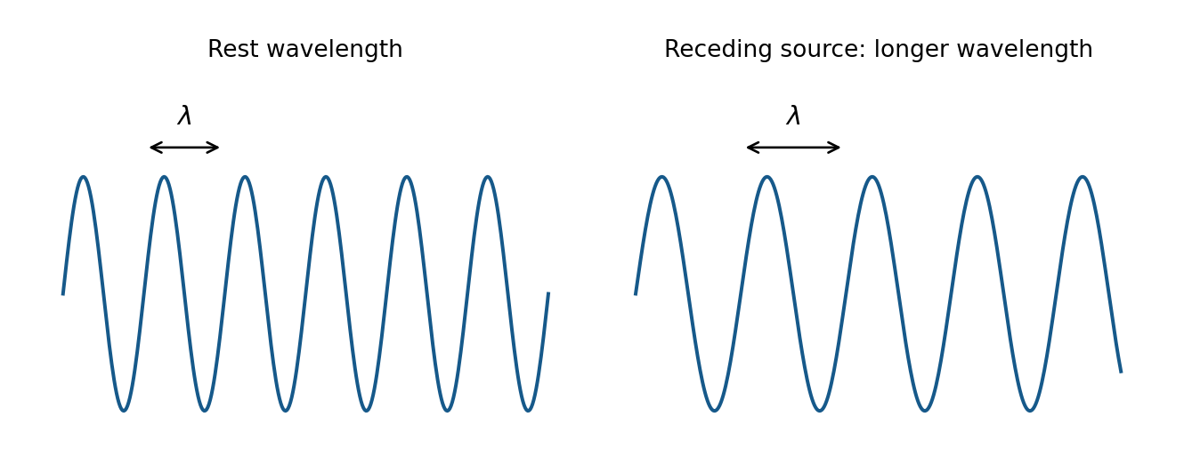
The panjang gelombang 波长$\lambda$ is the distance between nearest points vibrating in phase. The wave speed 波速$v$ is the speed at which a fixed phase, such as a crest, travels. It is not the speed of a vibrating particle.
A transverse wave 横波 has vibrations perpendicular to its direction of travel. A rope moves up and down while its disturbance travels along the rope.
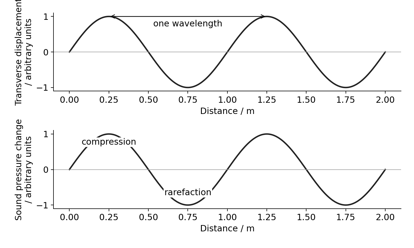
A longitudinal wave 纵波 has vibrations parallel to its direction of travel. Sound has compressions 密部, where pressure and density are higher, and rarefactions 疏部, where they are lower.
Air molecules move back and forth about their resting positions. They do not travel from the speaker to your ear with the sound.
Distance graphs show a whole wave at one instant.
Read the horizontal axis first
A displacement–distance graph is a snapshot. The separation of neighbouring crests gives $\lambda$. A displacement–time graph follows one particle. The separation of neighbouring peaks gives $T$. The same curve shape can represent either graph, but the quantities are different.
For a longitudinal wave, a pressure–distance graph shows compressions at pressure maxima. A molecular displacement–distance graph shows displacement along the direction of travel. Maximum compression occurs where displacement changes most rapidly towards the neighbouring molecules. Pressure maximum and displacement maximum are not at the same place; their patterns are one-quarter wavelength apart in a sinusoidal travelling sound wave.
Worked example. A microphone records 12 complete cycles in $0.030\ \text{s}$. Sound travels at $340\ \text{m s}^{-1}$. Find its frequency and wavelength.
Known: cycle count, total time and speed. Frequency counts cycles per second; the wave equation then links speed to wavelength.
Check: one cycle takes $T=1/f=0.0025\ \text{s}$. Twelve cycles take the stated $0.030\ \text{s}$.
Superposition and standing waves
A wavefront 波阵面 joins points at the same phase. Fasa 相位 describes the stage of a vibration cycle. One complete cycle corresponds to $360^\circ$ atau $2\pi$ radians.
Superposisi 叠加 means adding the displacements of overlapping waves at each point. Interferensi 干涉 is the resulting reinforcement or cancellation. Coherent sources 相干波源 have the same frequency and a constant phase difference. Their phase difference need not be zero.
For waves of the same wavelength, the phase difference caused by a path difference 路程差$\Delta x$ is:
For sources initially in phase, path differences $0,\lambda,2\lambda,\ldots$ give constructive interference. Half-integer wavelength differences give destructive interference. Complete cancellation also needs equal amplitudes. If sources start with a phase difference, include it too.
Worked example. Two in-phase speakers produce wavelength $0.80\ \text{m}$. Their paths to a microphone differ by $1.20\ \text{m}$.
Known: path difference and wavelength. Convert path difference into cycles, then phase.
$540^\circ$ is equivalent to $180^\circ$. The waves arrive in opposite phase and interfere destructively. The sound need not become silent if the arriving amplitudes differ.
How a standing wave forms
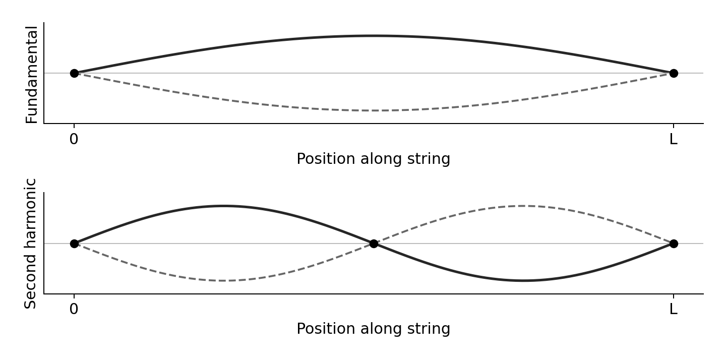
A standing wave 驻波 forms when two waves of the same frequency and similar amplitude travel in opposite directions and superpose. Reflection at a fixed string end supplies the returning wave.
A simpul 波节 always has zero displacement. An antinode 波腹 has the largest vibration amplitude.
Adjacent nodes are $\lambda/2$ apart. A node and its nearest antinode are $\lambda/4$ apart.
Points between the same pair of nodes vibrate in phase. Points in neighbouring sections vibrate in opposite phase.
All points have the same frequency, except that a node does not vibrate. Amplitude depends on position.
An ideal standing wave has no net energy transfer along it. A travelling wave carries energy along its direction of travel.
The end nodes remain still; the curve changes between the solid and dashed shapes.
For a string fixed at both ends, length $L$ contains a whole number $k$ of half-wavelengths:
$$L = \frac{k\lambda}{2} \qquad v = \sqrt{\frac{T}{\mu}} \qquad f = \frac{k}{2L}\sqrt{\frac{T}{\mu}}$$
Here $T$ is tension 张力, not period; $\mu$ is mass per unit length 线密度 in $\text{kg m}^{-1}$. The fundamental has $k=1$. At fixed mode, frequency increases with $\sqrt{T}$, decreases with $L$, and decreases with $\sqrt{\mu}$.
Worked example. A $0.60\ \text{m}$ string has $\mu=1.5\times10^{-3}\ \text{kg m}^{-1}$ and tension $24\ \text{N}$. Find its fundamental frequency.
Known: length, tension and linear density. The fundamental fits half a wavelength between the fixed ends.
Doubling tension multiplies frequency by $\sqrt{2}$, rather than by two.
Standing sound in a closed tube
In the simplest standing sound wave in a tube closed at one end, the closed end is a molecular displacement node. The open end is approximately a displacement antinode. This fits one-quarter wavelength into the effective tube length, so $L_{effective}=\lambda/4$. The pressure pattern is reversed: the closed end is a pressure antinode. Do not call a pressure node a displacement node. Real tubes have a small open-end correction; use an effective length if the question supplies it.
Worked example. A closed tube has effective length $0.20\ \text{m}$ and fundamental frequency $425\ \text{Hz}$. The end conditions give $\lambda=4L=0.80\ \text{m}$; then $v=f\lambda=425\times0.80=340\ \text{m s}^{-1}$. A string fixed at both ends instead fits half a wavelength in its fundamental. Choose from the end conditions, not from the word “standing”.
Core practical 4: speed of sound
Use a signal generator, speaker, movable microphone and two-beam oscilloscope 双踪示波器. Connect one oscilloscope channel to the generator reference signal and the other to the microphone output. Both traces have the same frequency.
Keep frequency constant. Move the microphone along a measured line away from the speaker. Find a position where the traces are in phase.
Move to another in-phase position. Consecutive in-phase positions are one wavelength apart. Measure across several wavelengths and divide by their number.
Read the period from the time-base scale: count horizontal divisions across several cycles, then divide. Find $f=1/T$ and use $v=f\lambda$.
Repeat positions and frequencies. Keep the microphone on the speaker axis. Reduce reflected sound by working away from walls. Measure position from a fixed microphone reference point.
Measuring several wavelengths reduces the percentage uncertainty in the distance. Measuring several periods does the same for time. A resonance-tube experiment can also measure sound speed, but it does not replace this specified practical.
Core practical 5: vibrating string
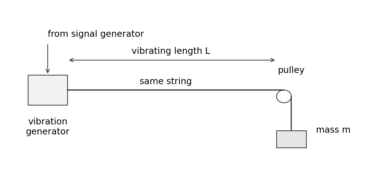
Use a vibration generator driven by a signal generator. Run the string over a pulley to a hanging mass. The tension is about $mg$ when pulley friction is small. Increase frequency until a clear standing-wave pattern forms.
Investigate tension: keep $L$, $\mu$ and mode fixed. Vary hanging mass. Plot $f^2$ melawan $T$; the gradient for the fundamental is $1/(4L^2\mu)$.
Investigate length: keep tension, string type and mode fixed. Plot $f$ melawan $1/L$.
Investigate linear density: measure string mass and length, $\mu=m/l$. Use different strings with fixed tension, vibrating length and mode. Plot $f^2$ melawan $1/\mu$.
Measure length between the end nodes. Find the resonance from both higher and lower frequencies and repeat. Secure the stand and keep clear of falling masses.
Intensity, refraction and polarisation
Intensity 强度 is power per unit area perpendicular to the energy flow:
$$I = \frac{P}{A}$$
Its unit is $\text{W m}^{-2}$. For a receiver, incident power is $P=IA$. Useful output is smaller if efficiency is below 100%. Convert area carefully: $1\ \text{cm}^2=10^{-4}\ \text{m}^2$.
Worked example. Radiation intensity is $800\ \text{W m}^{-2}$ over a $25\ \text{cm}^2$ solar cell. Efficiency is 20%. Can it supply $0.50\ \text{W}$?
Known: intensity, area, efficiency. First find incident power, then useful power.
$0.40\ \text{W}<0.50\ \text{W}$, so it cannot supply the required useful power.
Refraction and total internal reflection
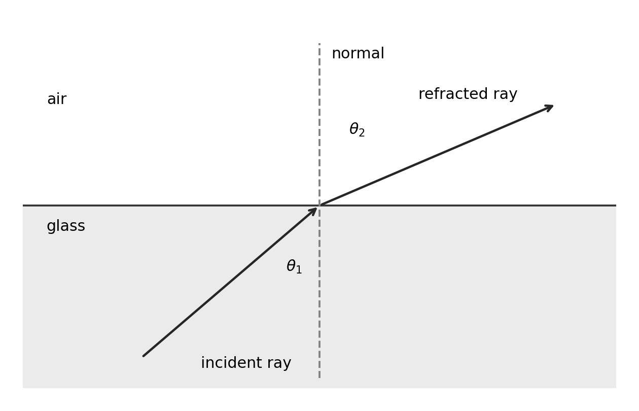
Pembiasan 折射 is a change in wave direction when speed changes at an interface. A ray entering along the normal changes speed without changing direction. The normal 法线 is perpendicular to the boundary. Measure all ray angles from it.
The refractive index 折射率$n$ compares vacuum light speed $c$ with speed in the material. Frequency stays constant across the boundary, so wavelength changes with speed. Entering higher $n$ bends the ray towards the normal; entering lower $n$ bends it away.
The ray bends away from the normal when it enters the lower-index medium.
Total internal reflection 全反射 requires travel from higher to lower refractive index and incidence greater than the sudut kritis 临界角$C$.
$$\sin C = \frac{n_2}{n_1} \qquad \text{for material to air: }\sin C = \frac{1}{n}$$
At $C$ the refracted angle is $90^\circ$; call incidence greater than $C$ total internal reflection. Below $C$, some energy is normally reflected and some transmitted. An optical fibre uses a higher-index core and lower-index cladding. Raising the cladding index raises the critical angle and can stop a previously reflected ray being trapped.
Worked example. Light travels from glass of index 1.50 into air. Does an incidence angle of $45^\circ$ produce total internal reflection?
Known: the two indices and incidence angle. Find the boundary angle before comparing.
The light travels towards lower index and $45^\circ>41.8^\circ$. Both conditions hold, so total internal reflection occurs.
Measuring refractive index
Place a rectangular transparent block on paper and trace its outline. Use a narrow ray-box beam. Mark two points on the incident ray and two on the emerging ray. Remove the block and join the boundary points to reconstruct the ray inside. Draw the normal at entry and measure incidence $i$ and refraction $r$ with a protractor.
Repeat for several incidence angles, keeping the same material and light colour. Plot $\sin i$ vertically against $\sin r$ horizontally. For air into the block, the gradient is the block's refractive index relative to air. Use a large triangle on a best-fit line. Narrow beams and widely separated ray marks reduce direction uncertainty. Very small angles give large percentage angle uncertainties.
Plane polarisation
Plane polarisation 平面偏振 restricts transverse vibrations to one plane containing the propagation direction. Unpolarised light has vibrations in many planes. A polariser transmits one vibration direction. Rotate a second polariser: parallel transmission directions give maximum brightness; perpendicular directions ideally give darkness. The ray still travels forward; its vibration direction changes selection.
Longitudinal waves cannot be plane polarised because their vibration is already along propagation. Polarisation is therefore evidence that light is transverse.
Diffraction and pulse-echo
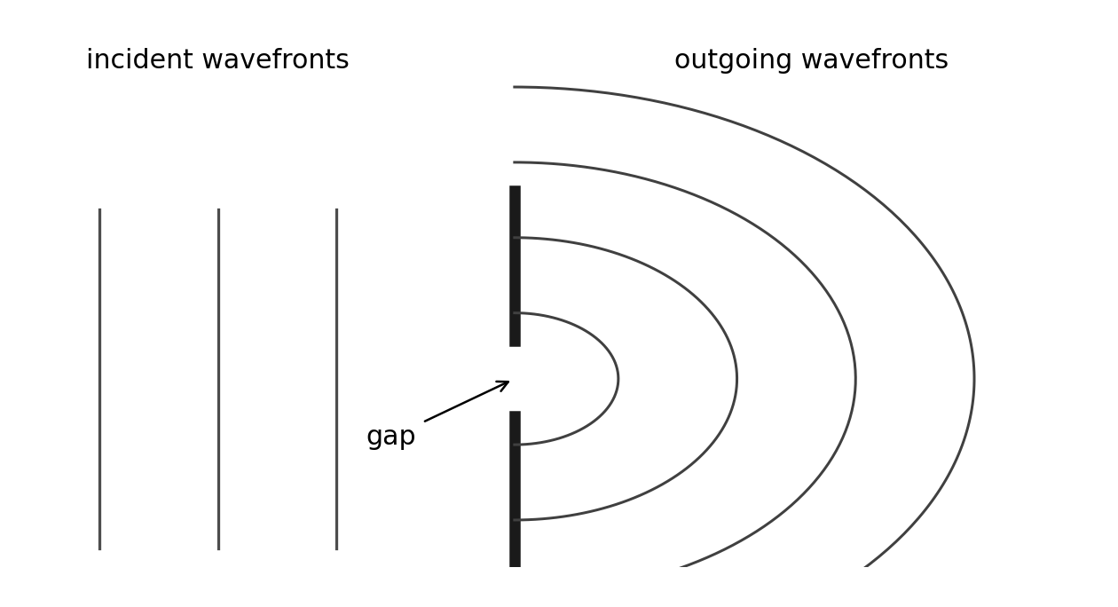
Difraksi 衍射 is the spreading of waves at a gap or edge. Spreading is greater when the gap width is comparable to the wavelength. A wide gap still diffracts at its edges, but the central wave spreads less.
In Huygens' construction 惠更斯作图法, each point on a wavefront acts as a source of secondary wavelets. Draw wavelets of equal radius after the same time. Their forward common tangent gives the new wavefront. At a narrow gap only a small part of the original front supplies wavelets, so the emerging fronts spread widely. This explains spreading without inventing a change of frequency at the slit.
The gap limits which points supply the outgoing wavelets.
Gratings and core practical 6
A diffraction grating 衍射光栅 contains many equally spaced slits. Bright maxima occur when contributions from neighbouring slits arrive in phase:
$$k\lambda = d\sin\theta$$
Here $k$ is the integer orde 级次, $d$ is slit spacing, and $\theta$ is measured from the straight-through direction. The equation assumes normal incidence. If the grating has $N$ lines per metre, $d=1/N$. Do not confuse grating order with refractive index; printed papers may use $n$ for either.
Worked example. A grating has 600 lines per millimetre. First-order light appears at $18.0^\circ$. Find its wavelength.
Known: line density and first-order angle. Convert line density before taking its reciprocal.
This is $515\ \text{nm}$. Check each proposed higher order using $k\lambda/d\leq1$.
For CP6, aim a low-power laser normally at a grating and place a screen perpendicular to the central beam. Measure screen distance $D$ and displacement $x$ from the central spot to an order. Use $\tan\theta=x/D$, then the grating equation. Average corresponding left/right displacements, repeat distances, and use higher visible orders where measurement is clear. Measure from the grating to the screen, not from the laser casing. Do not substitute $\sin\theta=x/D$ unless a justified small-angle approximation is acceptable. Never look into the beam; keep it below eye level and stop stray beams.
Electrons also show wave behaviour
An electron beam passing through a thin crystal produces a diffraction pattern. Regular atom spacing provides the diffracting structure. Changing electron momentum changes the pattern spacing. This is evidence of wave behaviour; particles travelling along simple straight paths alone cannot explain the diffraction maxima.
The de Broglie wavelength 德布罗意波长 is:
$$\lambda = \frac{h}{p}$$
For a non-relativistic electron, $p=mv$. If it gains kinetic energy by crossing a potential difference, $E_k=eV$ dan $p=\sqrt{2mE_k}$. Use these links only when the question gives or requires that energy relation.
Worked example. An electron has momentum $2.0\times10^{-24}\ \text{kg m s}^{-1}$. With $h=6.63\times10^{-34}\ \text{J s}$:
Increasing momentum reduces wavelength. Electrons have both particle and wave properties; diffraction does not mean that an electron becomes a sound wave.
Reflection, transmission and echoes
At an interface, part of a wave's energy may be transmitted 透射 and part reflected. A reflected pulse can locate a boundary. In pulse-echo 脉冲回波, measured delay includes the outward and return journeys:
$$2s = vt \quad\Rightarrow\quad s = \frac{vt}{2}$$
Worked example. Ultrasound travels in metal at $5900\ \text{m s}^{-1}$. An echo returns after $12\ \mu\text{s}$.
The boundary is $35\ \text{mm}$ away, not $71\ \text{mm}$. A nearby echo may overlap the transmitted pulse. Shorter pulse duration reduces this blind region and separates close echoes. Shorter wavelength helps detect or distinguish smaller features. These are related limits, but pulse duration and wavelength are not the same quantity. Use the speed in the actual material, not automatically the speed in air.
Foton dan efek fotolistrik
Wave ideas explain interference, diffraction and polarisation. They did not explain all observations of energy transfer. Foton 光子 describe discrete packets of electromagnetic energy:
$$E = hf = \frac{hc}{\lambda}$$
Historically, interference and diffraction supported wave models of light. Quantum ideas developed to explain observations including the photoelectric effect and atomic spectra. Modern physics uses both wave and photon descriptions according to the measurement. A successful new model must explain evidence that the older model explains too.
One photon and one electron
In the photoelectric effect 光电效应, a surface electron absorbs a photon and may escape. The work function 逸出功$\phi$ is the minimum energy needed to remove an electron from the surface. The threshold frequency 极限频率 is $f_0=\phi/h$.
Below threshold, increasing intensity does not cause emission in the usual single-photon model.
Above threshold, higher frequency raises maximum kinetic energy. A graph of $E_{k,\max}$ melawan $f$ has gradient $h$, frequency intercept $f_0$ and extrapolated energy intercept $-\phi$.
At fixed frequency above threshold, higher intensity supplies more photons per second. More electrons can be emitted per second, so the saturation photocurrent rises. Their maximum kinetic energy does not rise.
Emission starts without the energy-building delay predicted by a simple continuous-wave energy model, even at low intensity above threshold.
Electrons escape with a range of kinetic energies. Some lose more energy within the material. The equation describes the largest energy, not every electron's energy.
The electronvolt 电子伏特 is an energy unit: $1\ \text{eV}=1.60\times10^{-19}\ \text{J}$. It is not a unit of potential difference. A stopping potential $V_s$ just prevents even the fastest photoelectrons reaching the collector, so $eV_s=E_{k,\max}$.
Worked example. Light of frequency $8.0\times10^{14}\ \text{Hz}$ reaches a surface with work function $2.0\ \text{eV}$.
Known: photon frequency and work function. Convert the work function into joules before subtracting.
The positive kinetic energy confirms that this frequency is above threshold. A negative subtraction would mean no emission, not negative kinetic energy.
Atomic line spectra
Atoms have discrete energy levels 分立能级. An electron moving down between two allowed levels emits a photon. Moving up requires absorption of the matching energy:
$$|\Delta E| = hf = \frac{hc}{\lambda}$$
A line spectrum has particular frequencies because only certain level differences are allowed. The largest downward energy difference gives the highest frequency and shortest wavelength. Count possible transitions by checking level pairs and which upper levels are populated; do not automatically count the number of levels as the number of lines.
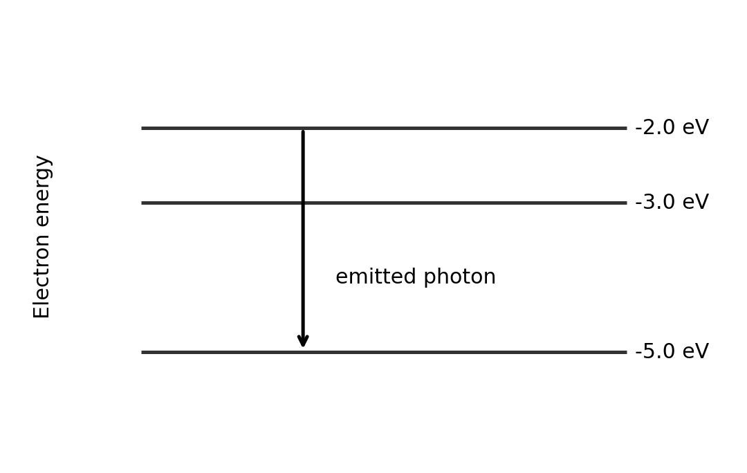
The photon energy equals the difference between the two levels.
Worked example. An electron drops from $-2.0\ \text{eV}$ ke $-5.0\ \text{eV}$.
Photon absorption in a material does not always eject an electron from its surface. Excitation followed by emission, for example in a light-activated material, is not automatically the photoelectric effect.
Current, resistance and circuits
Arus 电流 is the rate of charge flow. Conventional current follows the direction positive charges would move. In a metal, electrons drift in the opposite direction.
$$I = \frac{\Delta Q}{\Delta t} \qquad V = \frac{W}{Q} \qquad R = \frac{V}{I}$$
One ampere is one coulomb per second. Potential difference 电势差$V$ is energy transferred per unit charge between two points. Resistance $R$ is defined by the ratio $V/I$ at an operating point. Hukum Ohm 欧姆定律 is the extra condition $I\propto V$ when temperature and other physical conditions stay constant. Not every resistor or component obeys it.
Worked example. A current of $0.40\ \text{A}$ flows for $30\ \text{s}$. Find the number of electrons passing a point.
$$Q = It = 0.40\ \text{A}\times30\ \text{s} = 12\ \text{C}$$
Charge conservation 电荷守恒 means charge does not build up at a steady-current junction. Total current entering equals total current leaving. Current is not used up by a resistor.
Kekekalan energi 能量守恒 means the total energy supplied per coulomb around a complete loop equals the energy transferred per coulomb. The sum of voltage rises equals the sum of voltage drops.
For series resistors, the same current passes through each and their potential differences add:
A parallel combination has smaller resistance than its smallest branch resistance. A voltmeter connects in parallel across a component; an ideal voltmeter has infinite resistance. An ammeter connects in series; an ideal ammeter has zero resistance.
Worked example. A $6.0\ \Omega$ resistor is parallel to $3.0\ \Omega$. The combination is in series with $4.0\ \Omega$ across $12\ \text{V}$.
Known: circuit arrangement. Reduce the parallel section first, then apply the series rule.
Check: branch currents add to $2.0\ \text{A}$. The remaining series resistor has an $8.0\ \text{V}$ drop.
Power and component graphs
Daya listrik 电功率 is energy transferred each second. Substituting $V=IR$ ke dalam $P=VI$ gives the other forms:
$$P = VI = I^2R = \frac{V^2}{R} \qquad W = Pt = VIt$$
Use voltage across, and current through, the same component. The resistance forms apply to its operating-point resistance; do not assume a heating lamp has constant resistance.
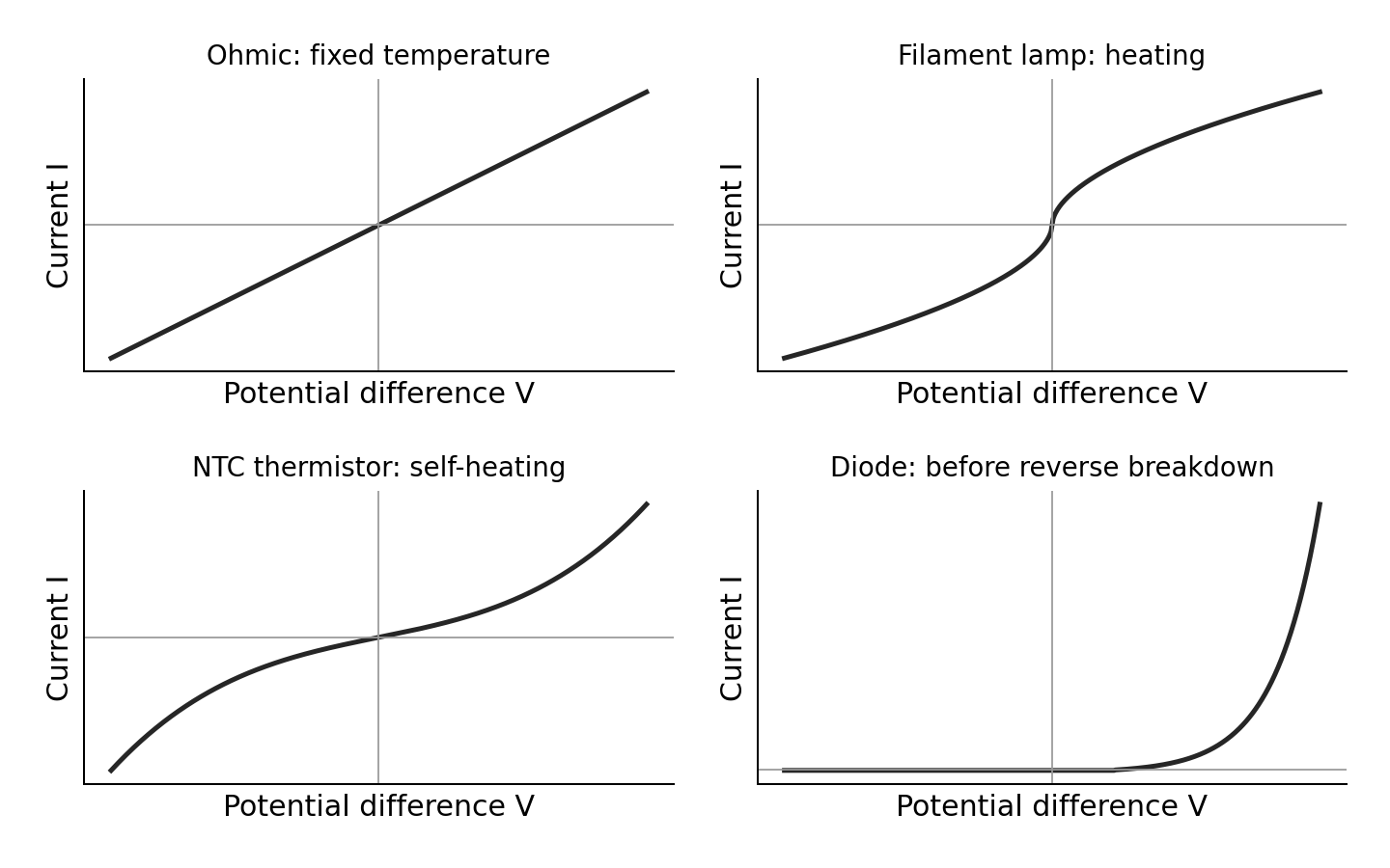
Axes and temperature conditions matter when interpreting these schematic curves.
Ohmic conductor at constant temperature: straight line through the origin. On an $I$-vertical, $V$-horizontal graph its gradient is $1/R$.
Filament lamp: as voltage magnitude rises, heating increases resistance. The $I$–$V$ curve becomes less steep.
NTC thermistor: heating lowers resistance. If current heats it sufficiently, the curve becomes steeper. At a controlled fixed temperature its behaviour over a suitable range can be approximately ohmic. Do not claim every thermistor curve must bend under every measurement condition.
Diode: very small reverse current before breakdown; forward current rises rapidly after a characteristic knee. It conducts mainly in one direction. A real diode does not have one constant resistance.
For a curved graph, $R=V/I$ uses a line from the origin to the operating point. The tangent gradient is not generally $1/R$.
Resistivity and core practical 7
Resistivity 电阻率$\rho$ is a material property at a stated temperature:
$$R = \frac{\rho l}{A} \qquad A = \frac{\pi d^2}{4}$$
Lengthening a uniform wire increases resistance. Increasing cross-sectional area decreases it. Doubling diameter gives four times the area and one-quarter the resistance, if material, length and temperature stay unchanged.
For CP7, connect a uniform wire, ammeter, power supply, switch and current-limiting resistor in series. Connect a voltmeter across the measured wire length. Measure several lengths and find $R=V/I$ for each. Plot $R$ melawan $l$: gradient $=\rho/A$, so $\rho=A\times\text{gradient}$.
Measure diameter with a micrometer at several positions and orientations; check its zero. Measure length between the actual electrical contacts. Use a small current and switch off between readings to limit heating. Keep contacts secure. A non-zero intercept may indicate contact or lead resistance. Repeating readings reduces scatter but does not remove a diameter zero error. Because area depends on $d^2$, a small percentage diameter uncertainty contributes about twice that percentage to area uncertainty.
Worked example. A wire diameter is $0.40\ \text{mm}$. An $R$–$l$ graph has gradient $3.5\ \Omega\,\text{m}^{-1}$.
The drift velocity 漂移速度$v$ is the small mean directed velocity of charge carriers, not their random thermal speed:
$$I = nqvA$$
Here $n$ is the number of mobile carriers per unit volume, $q$ is charge magnitude per carrier, and $A$ is cross-sectional area. A larger carrier density allows the same current with a smaller drift speed. In series wires the current is the same; changing $n$ atau $A$ changes $v$.
Materials have different resistivities because their carrier densities and the ease of carrier motion differ. More scattering reduces drift speed for the same applied potential gradient. Carrier density alone does not explain every difference between materials.
Potential dividers, sensors and cells
Along a uniform wire carrying steady current at constant temperature, resistance grows in proportion to distance. The potential drop therefore grows in proportion to distance too. A potential–distance graph is straight. This assumes uniform material and area; a tapered or unevenly heated wire need not give a straight line.
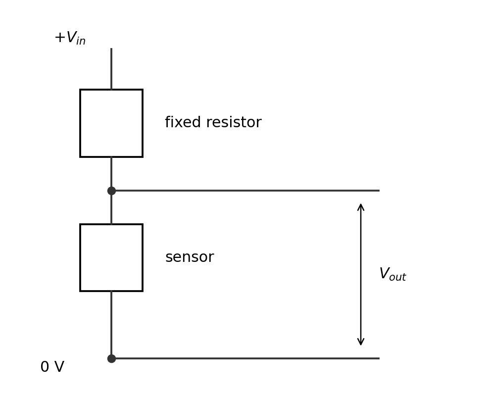
A potential divider 分压器 uses series resistances to share a supply voltage:
The expression assumes the output is unloaded, or the attached load draws negligible current. If a load draws significant current, combine it in parallel with the output resistor first. Always identify which resistor the voltmeter spans.
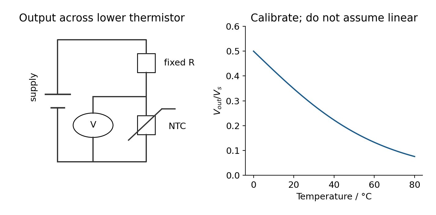
Swapping the sensor and fixed resistor reverses the direction of the output change.
Worked example. A $6.0\ \text{V}$ supply feeds a $2.0\ \text{k}\Omega$ fixed resistor above an LDR. Find the output across the LDR when its resistance changes from $4.0$ ke $1.0\ \text{k}\Omega$.
The output across this LDR falls when illumination rises. The output across the fixed resistor rises. Explain the named output, not just “the voltage changes”.
Explain sensors using carriers
In a metal, heating increases lattice vibrations. Conduction electrons scatter more often. The mobile electron number stays approximately constant, but drift speed at a given potential gradient decreases, so resistance rises.
Dalam sebuah negative-temperature-coefficient thermistor 负温度系数热敏电阻, heating releases more mobile carriers. The carrier-density increase dominates, so resistance falls. Avoid saying heating reduces lattice vibrations.
Dalam sebuah light-dependent resistor 光敏电阻 (LDR), absorbed light releases additional mobile carriers. Increased illumination raises carrier density and lowers resistance. It does not need to work by electrons leaving its surface.
For linked explanations, give the full chain: environmental change → carrier/scattering change → resistance change → divider fraction change → named output change. Keep the circuit arrangement in view throughout.
E.m.f., internal resistance and core practical 8
Electromotive force 电动势$\mathcal{E}$ is energy supplied by the source per unit charge. It is measured in volts, despite its name. Hambatan dalam 内阻$r$ causes energy transfer within the source when current flows. The terminal p.d. is the energy per coulomb available to the external circuit:
$$\mathcal{E} = V+Ir \qquad V = \mathcal{E}-Ir \qquad I = \frac{\mathcal{E}}{R+r}$$
The source supplies power $\mathcal{E}I$, the external circuit receives $VI$, and internal heating is $I^2r$. These add consistently. With negligible current, terminal p.d. approaches e.m.f.
For CP8, connect a cell, ammeter, variable load and switch in series. Connect a high-resistance voltmeter across the cell terminals. Vary the external resistance and record pairs of $V$ dan $I$. Plot $V$ vertically against $I$ horizontally. The best-fit line has intercept $\mathcal{E}$ and gradient $-r$. Take the magnitude of the gradient for $r$.
Use several settings and repeat. Open the switch between readings, avoid very small load resistance, and keep the cell temperature and charge state as steady as possible. Never short-circuit the cell. A graph that curves may show changing internal resistance or e.m.f.; do not force one fixed $r$ onto it without discussing the limitation.
Worked example. A cell graph passes through $(0.20\ \text{A},1.40\ \text{V})$ dan $(0.60\ \text{A},1.20\ \text{V})$.
Known: two points on the best-fit line. The gradient of $V=\mathcal{E}-Ir$ is $-r$.
Check using the second point: $1.20+0.60\times0.50=1.50\ \text{V}$ too. The terminal p.d. falls as current rises.
Cek diri sendiri
Use the matching exercise sheet after each section: 2.1 wave graphs; 2.2 standing waves; 2.3 refraction; 2.4 diffraction; 2.5 photons; 2.6 circuits; 2.7 dividers and cells.
Before using a past-paper set, check that you can:
read an axis and identify whether it gives wavelength, period, pressure or displacement;
explain a practical with apparatus, measurements, controlled variables, graph and precautions;
distinguish phase from amplitude, and photon frequency from photon arrival rate;
derive circuit combinations from charge and energy conservation;
explain a sensor circuit as a connected causal chain;
use an actual comparison to finish “deduce whether”, with units and a clear conclusion.
The reviewed January and June 2025 papers supply authentic examples, but do not test every requirement. Original practice fills the teaching gaps. Completing a sampled paper alone does not prove full syllabus coverage.
Pearson Edexcel IAL Physics Issue 3 (July 2021), printed pp.24–26 and Appendix 10 pp.75–77. These are local teaching subdivisions, not numbered official specification statements.
Plan an experiment: select apparatus and appropriate instrument range/resolution; discuss calibration and zero checks; describe correct measuring techniques; identify and control other relevant variables; judge whether repeated readings are appropriate; identify health/safety issues and practical precautions; explain data processing; identify uncertainty/systematic errors and ways to reduce or remove them; discuss benefits/risks and social, environmental or historical context.
Sumber: Silabus Cambridge International
3.2Measurement, recording and uncertainty
Pearson Edexcel IAL Physics Issue 3 (July 2021), printed pp.24–26 and Appendix 10 pp.75–77. These are local teaching subdivisions, not numbered official specification statements.
Implementation and measurements: assess number and range of readings; record significant figures consistently with resolution; inspect inconsistent readings rather than silently deleting them; read instruments, including Vernier calipers (0.1 mm) and micrometer screw gauge (0.01 mm); suggest specific additional apparatus or techniques to improve measurement. Determine single-reading percentage uncertainty using half instrument resolution, and repeated-reading uncertainty using half range. Apply the Appendix 10 meanings of accuracy, precision, repeatability, reproducibility, validity, error, uncertainty and resolution.
Sumber: Silabus Cambridge International
3.3Graphs, processing and justified conclusions
Pearson Edexcel IAL Physics Issue 3 (July 2021), printed pp.24–26 and Appendix 10 pp.75–77. These are local teaching subdivisions, not numbered official specification statements.
Processing results: calculate with appropriate significant figures and units; choose graph axes/scales and plot data; interpret the relationship and derive a constant from the graph using a large gradient triangle; propose realistic improvements; discuss uncertainty qualitatively/quantitatively; compare a measured interval with a proposed/accepted value. Unit 3 does not require compounding percentage uncertainties. Select a suitable range and targeted additional data near a maximum when the demand requires it.
Sumber: Silabus Cambridge International
Lembar Kerja
A number needs a method
Two groups measure the same wire. Their values differ. Which should you trust? You need more than the final number: the instrument, method, repeated readings and uncertainty all matter.
WPH13 Practical Skills in Physics I is a written paper about practical work from Units 1–2. It lasts 80 minutes and has 50 marks. All questions are compulsory. At least 20 marks assess mathematics at Level 2 or above. This guide supports real laboratory work; reading it does not replace making measurements yourself.
The three skill sheets follow the process: plan a valid investigation, collect and record measurements, then process results and justify conclusions. The official specification gives skill lists rather than numbered knowledge statements for this unit.
Planning a valid investigation
A valid measurement 有效测量 measures what you intend to measure. A precise timer does not help if it times the wrong event.
Start by naming the independent variable 自变量 that you change and the dependent variable 因变量 that you measure. List control variables 控制变量 that could also affect the dependent variable. Say how you will keep each important one steady.
Turn a description into a usable method
A method needs:
named apparatus, with a suitable measuring range and resolution 分辨率;
an arrangement showing where measurements are taken;
steps that another student can follow, including the start and end events;
several independent-variable settings over a useful range;
repeats where they test stability and estimate variation;
a calculation or graph that answers the investigation question;
specific sources of uncertainty and improvements;
realistic hazards with a practical way to reduce each risk.
Do not write only “take readings” or “use better equipment”. Name the reading, the instrument and what the improvement changes.
Worked planning example: string frequency and tension
Investigate how fundamental frequency depends on tension in a string.
Use a vibration generator and signal generator. Pass the string over a pulley to a mass hanger.
Change hanging mass $m$. With a freely moving pulley, tension is approximately $T=mg$.
Measure vibrating length between the end nodes. Use the same string and keep that length fixed.
Adjust frequency for the fundamental each time. The same mode is a control, not an optional detail.
Measure the string's mass and total length to find linear density $\mu$. Keep it unchanged in this investigation.
Record several tensions and their resonant frequencies. Repeat the tuning near each resonance.
A graph of $f^2$ vertically against $T$ horizontally should be straight through the origin. A large triangle gives the gradient. Secure the stand and keep your feet away from falling masses. This is stronger than saying “be careful”.
Calibration and zero checks
Calibration 校准 checks an instrument against known reference values. A zero error 零点误差 occurs when it does not read zero at the correct zero condition. Check closed micrometer jaws or an empty balance before measuring.
If a micrometer reads $+0.03\ \text{mm}$ with its jaws correctly closed, subtract $0.03\ \text{mm}$ from each subsequent reading. Repeating the measurement alone does not remove that offset. A zero check cannot prove that every point on the scale is calibrated correctly.
Range, spacing and repeats
Choose a range wide enough to reveal the relationship. Several measurements crowded near one setting may give a poor gradient. Use more settings near a turning point if you need to locate a maximum accurately.
Repeats are useful when conditions can be reproduced. They show scatter and help identify unstable readings. However, repeated readings of a discharging cell or a heating wire may drift because the conditions change. Reduce the current, switch off between readings, control temperature or restore conditions. Do not average a drift as though it were random variation.
Control the actual cause
When varying the angle of a lamp above a solar cell, keep lamp–cell distance and lamp output fixed. Control background light, for example with shielding or a darkened room. Keep the cell and its load the same. Otherwise a change in measured power may come from distance, illumination or circuit resistance instead of angle.
Discuss context using a physical cause. A tracking solar panel can stay closer to normal incidence and collect more energy over a day. Its motor also uses energy and adds cost or maintenance. “Better for the environment” alone does not explain either effect.
Measuring and recording
Accuracy 准确度 describes closeness to the true value. Precision 精密度 describes how closely repeated values cluster. Closely clustered results can still all share a systematic offset.
Repeatability 重复性 concerns similar results using the same operator and method over a short time.
Reproducibility 再现性 concerns similar results from different operators, apparatus or methods.
Random effects 随机影响 cause unpredictable variation. Repeating and taking a mean can reduce their influence.
Systematic error 系统误差 shifts results in a consistent way. Correct the cause or known offset; repeating does not remove it.
Uncertainty 不确定度 is a reasonable interval associated with a measurement. It is not automatically a mistake or the known size of the error.
Read instruments at their resolution
A millimetre ruler has a smallest interval of $1\ \text{mm}$. The specification's standard Vernier calipers resolve $0.1\ \text{mm}$, and its standard micrometer resolves $0.01\ \text{mm}$. Check the instrument shown: a digital display or a different scale may have a different resolution.
For a micrometer, add the visible sleeve reading and the thimble reading. Include a visible half-millimetre sleeve mark when appropriate. Use the ratchet for consistent contact pressure, rather than overtightening the jaws.
For Vernier calipers, read the main scale just before the Vernier zero, then add the aligned Vernier division times its resolution. Check that the jaws contact the intended surfaces without tilting. Do not infer a missing scale from an extracted text description: read the instrument diagram itself.
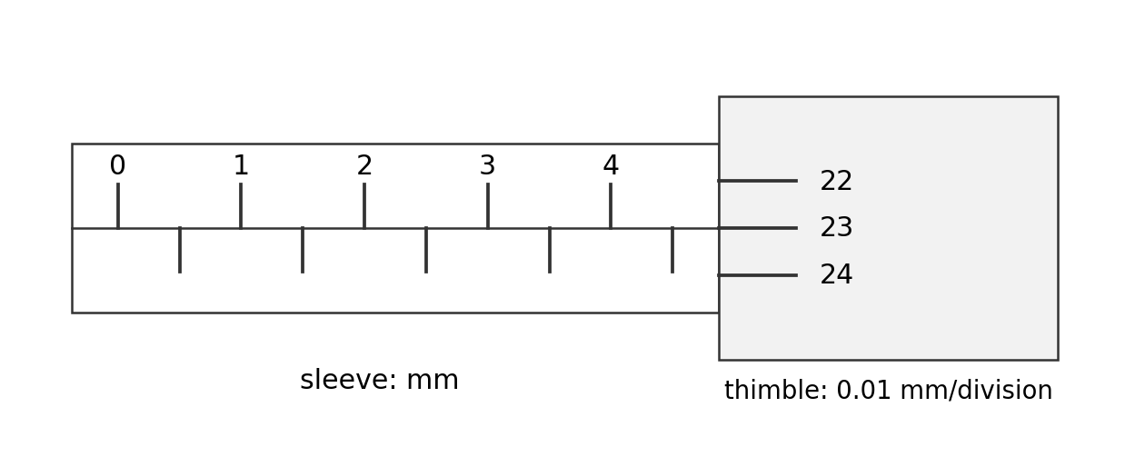
Read the sleeve before adding the aligned thimble division.
Worked example. The last visible sleeve mark is $4.5\ \text{mm}$. Thimble division 23 aligns with the reference line. Resolution is $0.01\ \text{mm}$ and zero error is $+0.02\ \text{mm}$.
Avoid parallax 视差 by viewing a scale along the correct line of sight. Use a set square to transfer a height or position onto a ruler. Keep the ruler parallel to the distance being measured; a sloping ruler measures a different distance.
A light gate measures the blocking time of an interrupting object. With known interrupting length $l$, speed is $v=l/t$. That gives speed during passage, not acceleration by itself. To find acceleration, measure a change of speed over known time, or use a justified motion equation with additional measured quantities. Do not call $l/t$ acceleration.
A video with known frame rate can reduce reaction-time uncertainty. Count frames between clearly defined start and end events, then use $t=N/f_{\text{frame}}$. The frame interval limits timing resolution. Blurred images or unclear event positions can still limit the result.
Tables and significant figures
Put quantity and unit together in each column heading, for example $l/\text{mm}$. Record raw measurements with decimal places matching instrument resolution. Do not add extra digits that the instrument cannot resolve.
Membaca
Time / s
1
5.12
2
5.24
3
5.18
4
5.20
These all have the same two decimal places. A calculated mean can be kept with extra digits during working, then reported sensibly. Processed values for plotting are commonly given to three significant figures, unless the question or data requires otherwise. Do not mix $5.1$, $5.24$ dan $5.180$ as if they came from one unchanged display.
An anomalous reading 异常读数 does not fit the pattern. Check the reading, method and repeat measurement if possible. Do not silently delete the least convenient value. A suspected anomaly needs a reason and a recorded decision.
Uncertainty in this unit
For one reading, this specification uses half the instrument resolution as the basic absolute uncertainty estimate. This does not mean resolution is the only source of uncertainty. A poorly defined endpoint, reaction time or alignment may make the uncertainty larger.
Report about $(5.19\pm0.06)\ \text{s}$. Keep the unrounded mean in the percentage calculation. The repeat spread is much larger than half a hundredth of a second, so quoting display resolution alone would miss the observed variation.
Unit 3 does not require compounding percentage uncertainties in a calculated quantity. If an uncertainty for that quantity is supplied, use it directly. Do not introduce an advanced propagation rule as a requirement here.
Graphs and processing results
Choose scales that show the data
Read which quantity belongs on each axis. Use clear quantity/unit labels and regular scales. Use a large part of the available grid; avoid awkward intervals that are hard to subdivide. Neither axis must always start at zero, but do not hide whether a proposed proportional relationship passes through the origin.
Plot small crosses accurately. Draw a thin best-fit line or smooth curve according to the relationship. Do not join noisy points with a zigzag unless the question requests it. A best-fit straight line balances scatter rather than passing through every point.
Use distant points on the best-fit line, not a tiny pair of neighbouring data points.
Turn a gradient into a physical constant
For a line $y=mx+c$, identify which part of the physical equation matches $m$ dan $c$. A straight line does not prove direct proportionality if its intercept is non-zero.
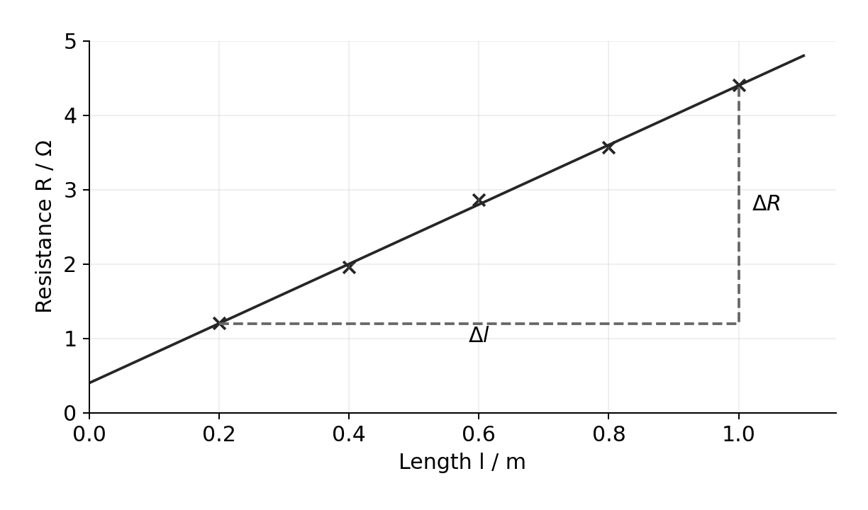
Worked example. A wire follows $R=(\rho/A)l+R_0$. A best-fit line passes through $(0.20\ \text{m},1.20\ \Omega)$ dan $(1.00\ \text{m},4.40\ \Omega)$.
Known: two widely separated points on the fitted line. Why: the slope equals $\rho/A$.
If $A=1.0\times10^{-7}\ \text{m}^2$, the resistivity is:
$$\rho = mA = 4.00\ \Omega\,\text{m}^{-1}\times1.0\times10^{-7}\ \text{m}^2 = 4.0\times10^{-7}\ \Omega\,\text{m}$$
The fixed intercept may represent contact or lead resistance. Dividing one measured $R$ by $l$ would include that offset and give the wrong slope.
Scale factors belong in the gradient
Suppose an axis is labelled $f/\text{MHz}$. A gradient read from that graph has MHz in its units. Convert to Hz before using SI constants. A graph of $f$ melawan $\sin\theta$ has a dimensionless horizontal axis; its gradient therefore has frequency units. Use degree mode if the measured angle is in degrees.
If a supplied equation is $f=(v/\lambda)\sin\theta$, a graph of $f$ melawan $\sin\theta$ has gradient $v/\lambda$. Rearrange $v=\lambda\times\text{gradient}$. Do not assume every frequency graph has gradient equal to speed.
Curves, maxima and specific improvements
A broad range first locates a maximum. Then take more closely spaced readings around that region. Repeating one point does not locate the maximum between existing points. Keep the other conditions steady, and consider scatter when quoting the best angle or resistance.
For a motion experiment, a set square can improve a horizontal-distance measurement. For a lamp experiment, a dark enclosure can reduce changing background illumination. For a resonance experiment, approach the loudest sound from both higher and lower frequencies and repeat. Each improvement targets a named limitation.
Conclusions supported by uncertainty
A value with uncertainty describes an interval. Compare that interval with the proposed value, then state what the evidence supports. Agreement within uncertainty does not prove that a material or model is uniquely identified.
Worked example. A measured density is $8.90\ \text{g cm}^{-3}$ with percentage uncertainty $0.9\%$. Could it agree with a proposed value $8.94\ \text{g cm}^{-3}$?
The interval is about $8.82$ ke $8.98\ \text{g cm}^{-3}$. The proposed value lies inside it, so the measurement is consistent with that value. It does not prove the object has that composition.
If two model predictions both lie inside the interval, the data does not distinguish them. Reduce the dominant uncertainty or add a different measurement before claiming a unique identification.
Cek diri sendiri
Before attempting a written practical problem, check that you can:
turn apparatus names into a usable method with controls and a processing route;
read resolution and correct a known zero offset;
distinguish accuracy, precision, repeatability and reproducibility;
calculate a mean, half range and percentage uncertainty;
plot data, use a large gradient triangle and interpret an intercept;
turn a supplied uncertainty into an interval and give a justified conclusion;
link each improvement to the measurement problem it actually reduces.
4.1Impulse and two-dimensional collisions (statements 81–86, CP9–10)
Pearson Edexcel IAL Physics WPH14/01, Issue 3 (July 2021), printed pp.28–31 (PDF pp.32–35).
Main-loop faithful paraphrase of numbered requirements; mathematical notation normalised from the original PDF. Local sheet boundaries are not official specification headings.
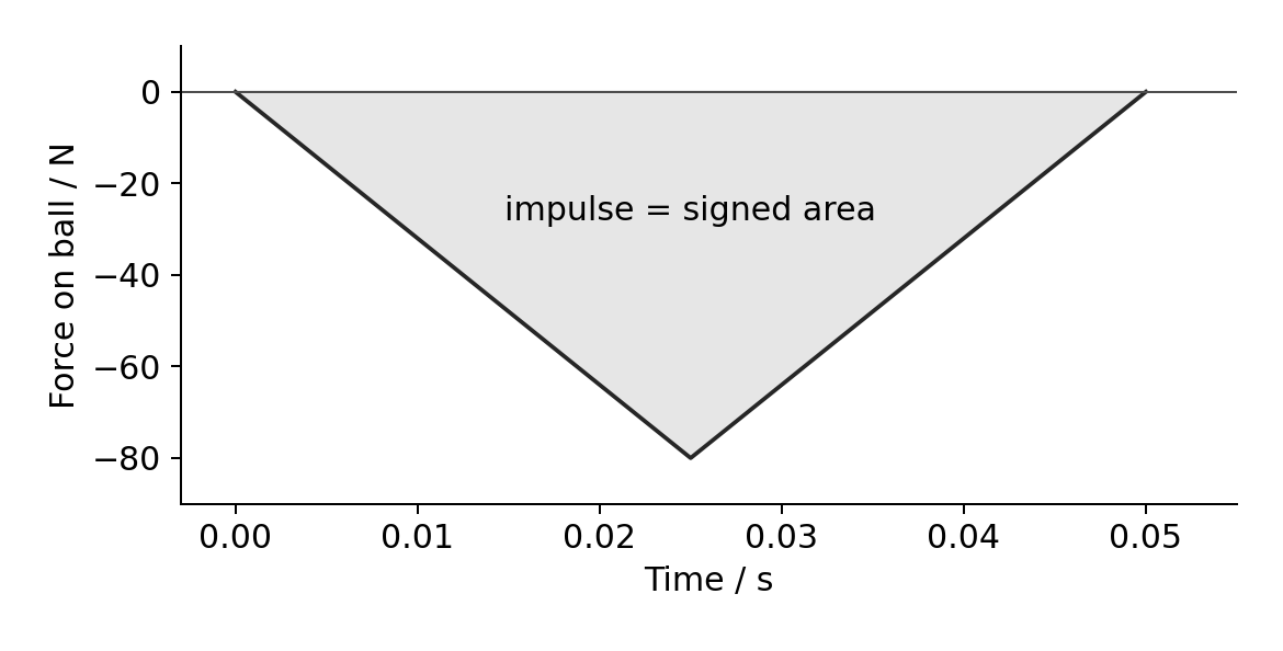
Understand and use impulse FΔt = Δp (Newton's second law).
CORE PRACTICAL 9: Investigate the force exerted on an object and its change of momentum.
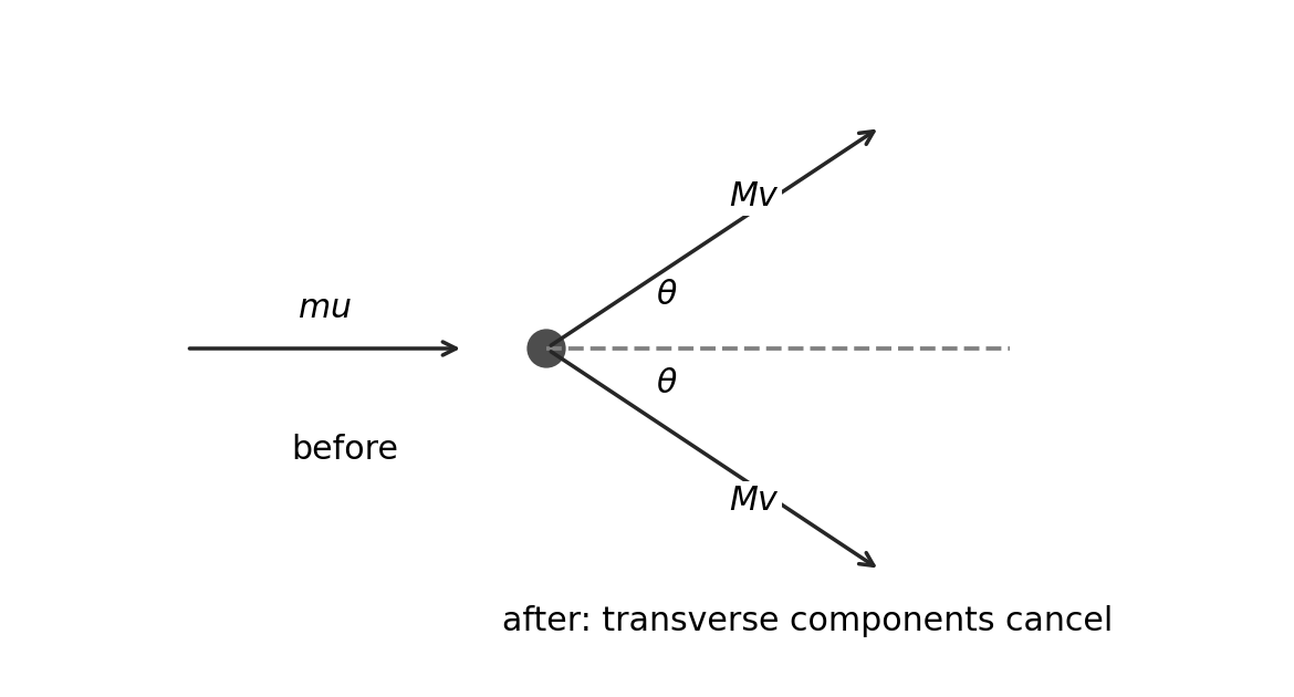
Apply conservation of linear momentum in two dimensions.
CORE PRACTICAL 10: Use ICT to analyse collisions between small spheres, such as ball bearings on a table top.
Determine whether a collision is elastic or inelastic.
Derive and use E_k = p²/(2m) for a non-relativistic particle.
Sumber: Silabus Cambridge International
4.2Circular motion (statements 87–91)
Pearson Edexcel IAL Physics WPH14/01, Issue 3 (July 2021), printed pp.28–31 (PDF pp.32–35).
Main-loop faithful paraphrase of numbered requirements; mathematical notation normalised from the original PDF. Local sheet boundaries are not official specification headings.
Express angular displacement in radians and degrees, and convert between them.
Understand angular velocity and use v = ωr and ω = 2π/T.
Use vector diagrams to derive a = v²/r = rω² and use these equations.
Understand that a resultant centripetal force produces and maintains circular motion.
Use F = ma = mv²/r = mrω².
Sumber: Silabus Cambridge International
4.3Electric fields and potential (statements 92–99)
Pearson Edexcel IAL Physics WPH14/01, Issue 3 (July 2021), printed pp.28–31 (PDF pp.32–35).
Main-loop faithful paraphrase of numbered requirements; mathematical notation normalised from the original PDF. Local sheet boundaries are not official specification headings.
Define an electric field as a region where a charged particle experiences a force.
Define and use electric field strength E = F/Q.
Use Coulomb's law F = Q₁Q₂/(4πε₀r²).
Use E = Q/(4πε₀r²) for a point charge.
Understand the relation between electric field and potential.
Use E = V/d for parallel plates.
Use V = Q/(4πε₀r) for a radial field.
Draw and interpret field lines and equipotentials for uniform and radial fields.
Sumber: Silabus Cambridge International
4.4Capacitors and RC circuits (statements 100–104, CP11)
Pearson Edexcel IAL Fisika WPH14/01, Edisi 3 (Juli 2021), dicetak hal.28–31 (PDF hal.32–35).
Parafraseta yang setia terhadap permintaan bernomor; notasi matematika dinormalisasi dari PDF asli. Batas lembar lokal bukan merupakan judul resmi dalam spesifikasi.
Definisikan kapasitansi C = Q/V dan gunakan persamaan tersebut.
Turunkan energi tersimpan W = ½QV dari area di bawah grafik beda potensial–muatan; turunkan dan gunakan W = ½CV² dan W = Q²/(2C).
Gambar dan tafsirkan kurva pengisian/pengosongan resistor–kapasitor dan pahami konstanta waktu RC.
PRAKTIK INTI 11: Gunakan osiloskop atau pencatat data untuk menampilkan dan menganalisis beda potensial kapasitor selama pengisian dan pengosongan melalui resistor.
Gunakan Q = Q₀ exp(−t/RC); turunkan dan gunakan persamaan arus dan beda potensial yang sesuai beserta bentuk logaritmiknya.
Sumber: Silabus Cambridge International
4.5Magnetic forces and induction (statements 105–110)
Pearson Edexcel IAL Fisika WPH14/01, Edisi 3 (Juli 2021), dicetak hal.28–31 (PDF hal.32–35).
Parafraseta yang setia terhadap permintaan bernomor; notasi matematika dinormalisasi dari PDF asli. Batas lembar lokal bukan merupakan judul resmi dalam spesifikasi.
Gunakan F = Bqv sinθ dan terapkan aturan tangan kiri Fleming untuk partikel bermuatan.
Gunakan F = BIl sinθ dan terapkan aturan tangan kiri Fleming untuk konduktor.
Pahami faktor-faktor yang mempengaruhi ggl induksi ketika kumparan dan magnet permanen bergerak relatif.
Pahami faktor-faktor yang mempengaruhi ggl induksi ketika arus berubah pada kumparan lain yang terkait.
Gunakan hukum Faraday dan persamaan gabungan Faraday–Lenz ggl = −d(Nφ)/dt.
Sumber: Silabus Cambridge International
4.6Nuclear structure, accelerators and tracks (statements 111–117, 120)
Pearson Edexcel IAL Fisika WPH14/01, Edisi 3 (Juli 2021), dicetak hal.28–31 (PDF hal.32–35).
Parafraseta yang setia terhadap permintaan bernomor; notasi matematika dinormalisasi dari PDF asli. Batas lembar lokal bukan merupakan judul resmi dalam spesifikasi.
Pahami nomor nukleon (massa) dan nomor proton (atomik).
Jelaskan bukti hamburan alfa sudut besar untuk model inti dan perubahan historis dalam model atom.
Pahami emisi elektron termionik dan percepatan menggunakan medan listrik dan magnet.
Pahami medan listrik/magnet pada linacs, siklotron, dan detektor; detail detektor dibatasi pada prinsip ionisasi dan pembelokan.
Turunkan dan gunakan r = p/(BQ) untuk partikel bermuatan dalam medan magnet.
Terapkan kekekalan muatan, energi, dan momentum pada interaksi partikel dan interpretasikan jejaknya.
Jelaskan mengapa energi tinggi diperlukan untuk menyelidiki struktur nukleon.
Pahami peningkatan waktu hidup partikel secara relativistik yang signifikan; persamaan relativistik tidak diperlukan.
Sumber: Silabus Cambridge International
4.7Particles, antiparticles and conservation (statements 118–119, 121–124)
Pearson Edexcel IAL Fisika WPH14/01, Edisi 3 (Juli 2021), dicetak hal.28–31 (PDF hal.32–35).
Parafraseta yang setia terhadap permintaan bernomor; notasi matematika dinormalisasi dari PDF asli. Batas lembar lokal bukan merupakan judul resmi dalam spesifikasi.
Gunakan ΔE = c²Δm dalam penciptaan dan annihilasi materi/antimateri.
Gunakan MeV/GeV untuk energi dan MeV/c² atau GeV/c² untuk massa serta konversi ke SI.
Klasifikasikan baryon (tiga kuark), meson (kuark/antikuarak), lepton fundamental, dan foton; ketahui bahwa simetri model memprediksi keberadaan kuark atas.
Gunakan sifat partikel untuk menyimpulkan sifat antipartikel yang sesuai dan sebaliknya.
Gunakan kekekalan muatan, bilangan baryon, dan bilangan lepton untuk menilai interaksi.
Tulis dan interpretasikan persamaan partikel dari simbol yang disediakan.
Sumber: Silabus Cambridge International
Lembar Kerja
From a collision to a particle accelerator
A car bumper and a particle detector seem very different. Both use momentum and forces. This unit follows those ideas into circular motion, electric fields, magnetic fields and particle interactions.
WPH14 assesses requirements 81–124 of the Issue 3 specification. It can also use knowledge from Units 1–2. Use the seven skill sheets in order. Check units, directions and the assumptions behind each equation. A familiar equation can give a wrong answer when its model does not fit.
Impulse and two-dimensional collisions
Force changes momentum
Momentum 动量 is the vector $\mathbf p=m\mathbf v$. Choose a positive direction before using signs. Impulse 冲量 is the change in momentum. For constant force, or the average force over an interval:
$$F_{\text{average}}\Delta t=\Delta p=m(v-u)$$
A changing force gives an impulse equal to the signed area under its force–time graph. A triangular pulse has area $\frac12\times\text{base}\times\text{height}$. An area below the time axis is negative. The maximum force is not automatically the average force.
Worked example. A $0.20\ \text{kg}$ ball approaches a wall at $+6.0\ \text{m s}^{-1}$. It rebounds at $-4.0\ \text{m s}^{-1}$. Contact lasts $0.050\ \text{s}$. Find average force on the ball.
Known: mass, signed initial/final velocities and contact time.
Why: force impulse changes the ball's momentum; rebound reverses the sign.
$$\Delta p=m(v-u)=0.20\ \text{kg}\times(-4.0-6.0)\ \text{m s}^{-1}=-2.0\ \text{kg m s}^{-1}$$
$$F_{\text{average}}=\frac{\Delta p}{\Delta t}=\frac{-2.0\ \text{kg m s}^{-1}}{0.050\ \text{s}}=-40\ \text{N}$$
The force is opposite the chosen positive direction. The wall feels an opposite force. A deforming bumper or helmet increases stopping time. For the same momentum change, this reduces average force. It does not remove the momentum change.
Conserve each momentum component
An isolated system 孤立系统 has no significant external impulse during the event. Its total momentum is conserved. Internal forces cancel in opposite pairs. Momentum conservation does not require kinetic energy conservation.
For a collision in a plane, resolve every momentum into two perpendicular axes:
Use the angle measured from the chosen axis. Include signs; a downward component is negative if upwards is positive. Do not add momentum magnitudes when directions differ.
Worked example. A $0.10\ \text{kg}$ sphere moving at $2.0\ \text{m s}^{-1}$ strikes two stationary spheres, each $0.10\ \text{kg}$. It stops. The two others leave symmetrically at $1.2\ \text{m s}^{-1}$, at angles $+\theta$ dan $-\theta$ to the original direction. Find their separation angle and classify the collision.
Why: transverse momenta cancel by symmetry; longitudinal momentum gives $\theta$.
An elastic collision 弹性碰撞 conserves total kinetic energy as well as momentum. An inelastic collision 非弹性碰撞 does not conserve kinetic energy; some becomes other forms of energy.
This collision is inelastic. Total energy is still conserved. In an ordinary passive collision, kinetic energy cannot increase without an additional energy source.
For a non-relativistic particle 非相对论粒子, use $p=mv$ dan $E_k=\frac12mv^2$. Substituting $v=p/m$ gives:
At equal kinetic energy, $p=\sqrt{2mE_k}$: a larger mass has larger momentum. At equal momentum, a larger mass has smaller kinetic energy. These equations are not valid for a particle moving close to light speed.
Core practicals 9 and 10
Untuk core practical 9, use a trolley, force sensor and data logger. Measure trolley mass and velocities just before/after contact using light gates or a motion sensor. Record the force–time pulse at a sampling rate fast enough to resolve it. Zero the force sensor; use consistent axes for force and velocity. Integrate the graph area and compare it with $m(v-u)$. Repeat for different contact forces or speeds. A graph of impulse against momentum change should have gradient close to one. Friction, sensor offsets and missed parts of the pulse can cause disagreement. Secure the track and catch the trolley safely.
Untuk core practical 10, record small spheres colliding on a level surface using an overhead camera. Include a length scale in the collision plane and a known frame rate. Keep the camera perpendicular to reduce perspective error. Track centres over several frames before and after the short collision. Convert pixel displacements to metres and frame intervals to seconds. Determine both velocity components, then compare total momentum components and kinetic energies. Repeat with different approach directions. Include uncertainty from positions, timing and scale calibration. A small mismatch within uncertainty is not evidence that momentum fails. Keep spheres contained so they cannot fall or become a slipping hazard.
Gerak melingkar
Angle, angular speed and tangential speed
An angle of one radian 弧度 subtends an arc equal to the radius. Hence $\theta=s/r$, with angle in radians. One revolution is $2\pi$ radians or $360^\circ$.
Angular velocity 角速度 describes the rate of angular displacement. In the plane problems here, use its signed rotational rate or magnitude as appropriate. Points on one rigid turntable have the same angular speed. Points farther from its centre have larger tangential speed 切向速率. Their velocity directions also vary around the circle.
Worked example. A wheel rotates at $120$ revolutions per minute. Find angular speed and acceleration of a point $0.25\ \text{m}$ from its centre.
Keep the unrounded angular speed during the calculation. Use radius, not diameter.
Why acceleration points inward
Uniform circular motion has constant speed but changing velocity. Draw the initial and final tangential velocity vectors. The change is $\Delta\mathbf v=\mathbf v_2-\mathbf v_1$, not their sum. For a small angular change, the velocity triangle and radius triangle are similar:
Centripetal force names the resultant of real forces. It is not an extra force to add to a force diagram. Friction can provide it on a turntable. Tension can provide it for a ball on a string.
Write the real-force equation
For clothing against the inside of a vertical drum, weight always points down. The drum's normal reaction points towards the centre. At constant speed:
The required resultant has the same magnitude, but the reaction is larger at the bottom. If contact is lost, the surface cannot provide a pulling normal reaction. Check this before using a circular-path model.
For a horizontal turntable, the largest available friction must be at least $mr\omega^2$. If maximum friction is $mg/25$:
Mass cancels because both required and available forces scale with mass. If the inward force disappears, motion initially follows the tangent. Gravity can then curve the later path; “tangent” describes the release direction.
Electric fields and potential
Force and potential describe different things
An electric field 电场 is a region where a charged particle experiences a force. Electric field strength 电场强度 is force per unit positive test charge:
Potential is a scalar; field is a vector. A point with zero potential need not have zero field. Adding signed potentials is different from adding field vectors.
Radial and uniform fields
For point charges, or outside an isolated charged conducting sphere, with $k=1/(4\pi\varepsilon_0)$:
Here $r$ is separation of charge centres; sphere distances are measured from its centre. Like charges repel, unlike charges attract. Potential takes the sign of $Q$ when zero is at infinity.
Between large parallel plates, away from edges, the field is approximately uniform:
$$|E|=\frac{|\Delta V|}{d}$$
The field points from higher to lower potential. Plate separation $d$ is perpendicular to the plates. An equipotential 等势面 has the same potential everywhere. Field lines cross equipotentials at right angles. Moving along one involves no change in electric potential energy.
The radial field is the negative potential gradient: $E_r=-\mathrm dV/\mathrm dr$. For a positive source, the signed area under its $E$–$r$ curve from $r$ to infinity equals $V(r)$. The area from zero to $r$ is not that potential. In a uniform field, closer equally spaced potential levels mean stronger field.
Worked example. A sphere of radius $0.20\ \text{m}$ has potential $9.0\ \text{kV}$. Find charge and field at $0.30\ \text{m}$ from its centre. Use $k=8.99\times10^9\ \text{N m}^2\text{C}^{-2}$.
Use the surface radius to find charge, then the new centre-distance to find field. Do not reuse the surface distance for the second step.
Compare electrical and gravitational forces
A stationary charged oil drop can satisfy $|q|E=mg$. Use $m=\rho\mathcal V$ if density and volume are given. Divide the charge magnitude by $e=1.60\times10^{-19}\ \text{C}$ to test whether it is close to an integer multiple. Charge sign follows the direction of force required, not its magnitude alone.
To lift a spherical grain, compare $qE$ with $\rho(4\pi r^3/3)g$. Radius is half the listed diameter. A calculated maximum diameter is a threshold: choose the largest listed diameter below it. On an inclined panel, the normal component of weight is $mg\cos\theta$. The electric force perpendicular to the panel need overcome that component to detach a grain; gravity also has a downslope component.
Capacitors and RC circuits
Charge storage and energy
A kapasitor 电容器 stores separated charge on two conductors. They carry equal and opposite charges in the ideal two-plate model. The quoted charge $Q$ is the magnitude on either plate, not the sum of both magnitudes. Kapasitansi 电容 is charge stored per unit p.d.:
$$C=\frac QV$$
One farad is one coulomb per volt. For constant capacitance, a $V$–$Q$ graph is straight through the origin with gradient $1/C$. Its area gives the work needed to transfer charge onto the capacitor:
$$W=\frac12QV=\frac12CV^2=\frac{Q^2}{2C}$$
The factor one half appears because p.d. rises from zero while charge is transferred. It is not $QV$ at the final voltage throughout charging. For discharge between non-zero voltages, subtract the two stored energies:
This is different from $\frac12C(V_{\text{initial}}-V_{\text{final}})^2$.
Charging and discharging
In an ideal series resistor–capacitor charging circuit, initially uncharged, the capacitor p.d. is zero. The resistor initially has the full supply p.d., so current is maximum. As charge builds, capacitor p.d. rises. Resistor p.d. and current fall. At full charge, current is zero and capacitor p.d. equals supply p.d.
For discharge through a fixed resistance, use signed current consistently or work with its magnitude:
The voltage relation follows from $Q=CV$ with constant $C$. Current magnitude follows from $|I|=V/R$ with constant $R$. The time constant 时间常数 is $\tau=RC$. After one time constant, $Q$, $V$ and current magnitude are $e^{-1}\approx0.368$ of their initial values. After three time constants they are about $5\%$, not zero. Stored energy falls faster because it depends on $V^2$.
A charging capacitor voltage rises towards $V_s$; charging current falls towards zero. Do not sketch the same curve for both quantities. Equal $V_C$ dan $V_R$ means each is $V_s/2$, reached at $t=RC\ln2$.
Taking natural logs of the discharge equation gives:
$$\ln V=\ln V_0-\frac{t}{RC}$$
Thus a graph of $\ln V$ melawan $t$ has gradient $-1/(RC)$ and intercept $\ln V_0$. The same forms hold for $Q$ and current magnitude. Use consistent measurement units inside the logged numerical values.
Worked example. A $100\ \mu\text{F}$ capacitor discharges from $12.0\ \text{V}$ through $20.0\ \text{k}\Omega$. Find p.d. after $3.0\ \text{s}$ and energy lost.
The lost stored energy becomes mainly heat in the discharge resistance. Use unrounded voltage in the final calculation.
Core practical 11 and useful extensions
Use a low-voltage d.c. supply, resistor, capacitor and switch. Charge through the resistor, then disconnect the supply and discharge through the known resistance. Connect a voltage sensor, data logger or oscilloscope across the capacitor. Record time and p.d.; choose a sampling interval short compared with $RC$. Use an instrument input resistance large compared with the discharge resistance, otherwise it changes the discharge path.
Pertahankan $R$ dan $C$ fixed, repeat after restoring the same initial charge, and compare measured curves with exponential predictions. Determine $RC$ from the $1/e$ level or a log-fit gradient. Avoid taking logs of readings near zero where relative uncertainty is large. For a resistance-tolerance test, calculate $R=-\Delta t/[C\ln(V_2/V_1)]$ during one uninterrupted discharge and compare with both limits of the permitted interval.
Use correct polarity for an electrolytic capacitor and remain below its voltage rating. Discharge it safely through a resistor before altering connections; do not short a charged capacitor. Leakage, sensor loading and resistor heating can change the measured curve.
A smoothing capacitor charges near supply peaks and discharges into the load between them. A smaller load resistance gives a smaller time constant, faster discharge and less smoothing. For two identical series capacitors, the same magnitude of charge appears on each. Their equal p.d.s share the supply, so each stores half the charge of one identical capacitor connected alone. This sharing is a useful bridge to the selected paper; it does not replace the main capacitance model.
Magnetic forces and induction
Directions, flux and force
Magnetic flux density 磁感应强度$B$ describes the field's force effect. For a straight wire of length $l$ in a uniform field:
$$F=BIl\sin\theta$$
Here $\theta$ is between conventional current and field. Only the length inside the field counts. For one charged particle:
$$F=|q|vB\sin\theta$$
Use Fleming's left-hand rule 弗莱明左手定则: first finger along field, second along conventional current, thumb gives force. A positive charge moves with conventional current. Reverse the result for an electron's motion. Dot symbols mean out of the page; crosses mean into it.
Magnetic force is perpendicular to velocity, so it changes direction without doing work. It cannot, alone, increase the particle's kinetic energy. If $\mathbf v$ is parallel to $\mathbf B$, magnetic force is zero.
Magnetic flux 磁通量 through a flat area in a uniform field is:
$$\phi=BA\cos\alpha$$
Here $\alpha$ is between field and the area's normal, not the plane itself. The unit is the weber. Flux linkage 磁通链 is $N\phi$ when the same flux links each of $N$ turns.
Worked example. A coil has 40 turns and radius $0.015\ \text{m}$. A uniform $0.020\ \text{T}$ field is perpendicular to its plane. Find flux linkage.
Use radius, not diameter, and multiply by turns only when finding linkage. A balance under magnets measures the opposite reaction to a force on a separately supported wire. Convert a balance reading change $\Delta m$ to force $\Delta mg$, not $\Delta m$ itself.
A changing linkage induces an e.m.f.
Induksi elektromagnetik 电磁感应 occurs when flux linkage changes. Relative movement of a coil and magnet can cause it. Rotating the coil or changing current in another linked coil can also cause it. A stationary coil in a constant field has no induced e.m.f. merely because flux is present.
Faraday's law 法拉第电磁感应定律 relates e.m.f. magnitude to rate of flux-linkage change. Lenz's law 楞次定律 gives the opposing direction:
Induced current, if the circuit is closed, produces a magnetic effect opposing the change that caused it. It does not always oppose the existing field: when that field decreases, the induced effect helps maintain it. This opposition is consistent with energy conservation.
Worked example. Flux through each of 50 turns decreases from $6.0\times10^{-5}$ ke $2.0\times10^{-5}\ \text{Wb}$ in $0.020\ \text{s}$. Find average induced e.m.f. magnitude.
Faster movement, stronger field, more turns or larger linked area can increase the rate. Explain which quantity actually changes. In a magnetic-strip reader, reversing pole orientation reverses signal direction. For a straight boundary swept across an area of width $L$ at speed $v$, $\Delta A/\Delta t=Lv$, giving $|\mathcal E|=NBLv$ under that uniform-field model.
Wireless charging uses alternating current in one coil, producing changing magnetic field and changing linkage in the phone coil. That induces an e.m.f. The receiving circuit can then charge the battery. Equal turn counts do not ensure equal voltages: some flux may fail to link the other coil, especially with separation or without an iron core.
Nuclear structure, accelerators and tracks
The nucleus and scattering evidence
In $^{A}_{Z}X$, proton number 质子数$Z$ counts protons and nucleon number 核子数$A$ counts protons plus neutrons. The neutron count is $A-Z$. A neutral atom has $Z$ electrons; an ion need not.
The older distributed-positive-charge model could explain small deflections but not the observed rare large-angle alpha scattering. Most alpha particles pass nearly straight through thin foil, showing that most of the atom is empty space. A small fraction experience very large deflections. Positive alpha particles feel strong electrostatic repulsion near a small, dense, positive nucleus containing most atomic mass. Few large-angle events show that the nucleus occupies a small fraction of the atom's volume. Keep each observation linked to the particular conclusion it supports.
Make, accelerate and steer a beam
Thermionic emission 热电子发射 releases electrons from a heated metal. Heating supplies energy so some electrons can leave the surface. A positive accelerating electrode attracts them through a vacuum. A potential difference changes kinetic energy by the electric work:
For speed calculations use the positive energy gain $|q|\,|\Delta V|$ only when the particle is accelerated through the field in the appropriate direction. Starting from rest, well below light speed:
$$\frac12mv^2=|q|\,|\Delta V|$$
A linear accelerator 直线加速器 uses alternating p.d. across gaps between drift tubes. Particles accelerate in gaps and are shielded inside the conducting tubes. The polarity reverses while particles are inside, so the next gap accelerates them again. At constant alternating frequency, increasing speed requires longer tubes to maintain the time between successive gaps. Across $n$ equal accelerating gaps, total kinetic-energy gain is $n|q|V_{\text{gap}}$.
A cyclotron 回旋加速器 uses a magnetic field perpendicular to two hollow dees. Electric field accelerates particles across the gap. Inside a dee, magnetic force curves the path without increasing speed. Polarity reverses during each half-turn, allowing another energy gain at the next crossing. With perpendicular entry:
In the non-relativistic model, the period is independent of speed. Increasing speed increases radius. Time in one dee is $T/2$, not $T$. The formula assumes constant field and fixed mass in this model; synchronisation fails as relativistic effects become important.
Worked example. A proton moves perpendicular to $B=0.40\ \text{T}$ with momentum $2.0\times10^{-20}\ \text{kg m s}^{-1}$. Use proton mass $1.67\times10^{-27}\ \text{kg}$.
When starting instead from a de Broglie wavelength, use $p=h/\lambda$, then $E_k=p^2/(2m)$ dan $V=E_k/|q|$. Check that the non-relativistic assumption remains suitable.
Read detector evidence carefully
Charged particles ionise matter along their paths, leaving detectable tracks. A neutral particle does not make a direct ionisation track in this model. Its presence can be inferred from missing momentum or from charged products it later produces.
In a known perpendicular magnetic field, curvature direction together with travel direction can identify charge sign. Without field direction, curvature alone cannot give sign. Radius gives momentum through $p=B|q|r$; comparing radii requires knowledge of charge magnitude. A tightening track often shows momentum being lost. Do not infer travel direction from a constant-radius arc alone.
Conserve charge, total energy and vector momentum at an interaction. If visible outgoing momenta do not add to the incoming momentum, a neutral product may carry the missing component. Draw a vector balance rather than guessing from the number of tracks.
High energies probe nucleon structure in two ways. Large momentum gives a short de Broglie wavelength, allowing small structure to be resolved. High collision energy also allows new massive particles to be created. Quarks are not observed as isolated free particles; do not describe a high-energy collision simply as removing a free quark.
Fast muons can reach the ground because their average lifetime measured in the Earth's frame is increased at speeds close to $c$. This does not mean they exceed light speed. Unit 4 requires the significance of this lifetime increase, not use of relativistic equations.
Particles, antiparticles and conservation
Families and antiparticles
In the quark–lepton model 夸克—轻子模型, baryons and mesons contain quarks. Leptons are fundamental particles in the model.
A baryon 重子 contains three quarks, for example a proton $uud$ or neutron $udd$. An antibaryon contains three antiquarks.
A meson 介子 contains one quark and one antiquark, for example a pion.
A lepton 轻子 is fundamental, for example an electron or neutrino. A positron is an antilepton, not a meson.
A photon is the quantum of electromagnetic radiation; it is neither a baryon nor a lepton.
Up-type quarks have charge $+2e/3$ and down-type quarks $-e/3$. Antiquarks have opposite charges. For example, $uud$ sums to $+e$ dan $udd$ to zero. The symmetry of the quark families predicted a top quark before it was observed. Classification models make testable predictions, not just lists of known particles.
An antiparticle 反粒子 has the same rest mass as its particle and opposite electric charge when charged. Other relevant additive quantum numbers also reverse. An electron has lepton number $+1$; its positron has $-1$. Both have baryon number zero. A neutral antiparticle can differ in quantum numbers despite having no electric charge.
Check conserved totals
Assign baryon number $+1$ to a baryon, $-1$ to an antibaryon, and zero to mesons/leptons/photons. Quarks carry $+1/3$ and antiquarks $-1/3$. Assign lepton number $+1$ to a lepton and $-1$ to an antilepton. Compare total charge, baryon number and lepton number on both sides of a proposed reaction. Also check energy and momentum. Passing the listed conservation checks alone does not prove that an interaction will occur; it establishes that those laws do not forbid it.
Worked example. Ujian $n\rightarrow p+e^-+\bar\nu_e$.
Jumlah
Before
After
Charge / $e$
0
$+1-1+0=0$
Baryon number
1
$1+0+0=1$
Lepton number
0
$0+1-1=0$
The antineutrino balances the electron's lepton number. Changing it to a neutrino would make the final total $+2$, so that proposed equation would fail this check. Preserve bars and charge signs when interpreting supplied particle symbols.
Rest energy, creation and annihilation
Mass–energy equivalence 质能等价 relates a rest-mass change to energy:
$$\Delta E=c^2\Delta m$$
In pair production 粒子对产生, energy creates a particle–antiparticle pair. The energy must at least supply both rest masses; extra energy can become kinetic energy or recoil. Momentum must also be conserved, so the surrounding interaction matters. In annihilation 湮灭, particle and antiparticle can turn into photons. A pair initially at rest producing two photons gives equal photon energies and opposite momenta. Each photon carries one particle's rest energy for an equal-mass pair; the total is twice that value.
One electronvolt is $e$ joules: $1\ \text{eV}=1.60\times10^{-19}\ \text{J}$. MeV means $10^6$ eV and GeV means $10^9$ eV. A quoted mass in $\text{MeV}/c^2$ is a mass unit, not an energy unit. Multiply by $c^2$ to get its corresponding rest energy.
Worked example. Convert a mass of $140\ \text{MeV}/c^2$ to kilograms.
Use the same units before comparing masses. Percentage difference from an accepted value is $100\times|m_{\text{predicted}}-m_{\text{accepted}}|/m_{\text{accepted}}$. State the reference value. In threshold questions, distinguish rest-energy supply from kinetic energy; do not use $p=mv$ for a photon or a particle close to $c$.
Cek diri sendiri
Can you use signed impulse and two momentum components, then test kinetic energy separately?
Can you derive centripetal acceleration and draw only actual forces?
Can you distinguish field vectors, signed potential and energy changes?
Can you choose the correct capacitor curve and use log slope or tolerance evidence?
Can you explain induction as a change in linkage, including the opposing direction?
Can you separate electric acceleration from magnetic steering and halve a cyclotron period correctly?
Can you preserve particle symbols, conservation totals and energy/mass units?
The skill sheets develop these methods before authentic past-paper tasks. Original practice also covers requirements not sampled in the two recent papers. A short sample of authentic questions does not define the whole syllabus.
Kalor spesifik/kalor laten; energi dalam; bedakan perpindahan energi dengan suhu. Kalibrasi termistor/pembagi potensial CP12 dan kalor laten CP13 dengan input listrik, kehilangan massa, dan koreksi kehilangan.
Permintaan bukti mundur: plans/2026-10-09-edexcel-ial-physics-u5-demand-map.md. Penilaian Unit 5 bersifat sinkopik dengan Units 1, 2, dan 4.
Sumber: Silabus Cambridge International
5.2Ideal gases and molecular kinetic energy (129–132, CP14)
Nol mutlak dan kelvin; pV=NkT, rasio jumlah tetap; CP14 tekanan/volume pada suhu tetap; turunkan energi kinetik translasi molekul rata-rata 3kT/2 dari teori kinetik, bedakan kecepatan RMS dan kecepatan kuadrat rata-rata.
Permintaan bukti mundur: plans/2026-10-09-edexcel-ial-physics-u5-demand-map.md. Penilaian Unit 5 bersifat sinkopik dengan Units 1, 2, dan 4.
Defisit massa dan energi ikat nuklir, konversi satuan u ke SI, grafik per-nukleon dan kestabilan, energi fusi/fisi, serta persyaratan suhu tinggi dan kepadatan untuk fusi berkelanjutan.
Permintaan bukti mundur: plans/2026-10-09-edexcel-ial-physics-u5-demand-map.md. Penilaian Unit 5 bersifat sinkopik dengan Units 1, 2, dan 4.
Sumber: Silabus Cambridge International
5.4Radiation, background and decay (137–142, CP15)
Pengurangan latar belakang; penetrasi dan ionisasi partikel alfa/beta/gamma; persamaan nuklir; serapan gamma oleh timbal dengan geometri tetap CP15; peluruhan spontan/lishu, aktivitas, waktu paruh, serta persamaan eksponensial dan logaritmik.
Permintaan bukti mundur: plans/2026-10-09-edexcel-ial-physics-u5-demand-map.md. Penilaian Unit 5 bersifat sinkopik dengan Units 1, 2, dan 4.
Sumber: Silabus Cambridge International
5.5Simple harmonic motion, graphs and energy (143–147, 149–150, CP16)
Restoring resultant proportional and opposite to displacement; signed x,v,a relations and phase, spring/pendulum periods, graph gradients, undamped energy exchange and damped energy loss. CP16 unknown mass from resonant frequencies with calibrated known masses.
Backward demand evidence: plans/2026-10-09-edexcel-ial-physics-u5-demand-map.md. Unit 5 assessment is synoptic with Units 1, 2 and 4.
Sumber: Silabus Cambridge International
5.6Forced oscillations, resonance and damping (148, 151–153)
Osilasi bebas versus osilasi paksa; frekuensi alami/pemacu, resonansi/pertukaran energi; kurva amplitudo-frekuensi dan redaman kualitatif; kerja resistif dan deformasi plastis duktil.
Permintaan bukti mundur: plans/2026-10-09-edexcel-ial-physics-u5-demand-map.md. Penilaian Unit 5 bersifat sinkopik dengan Units 1, 2, dan 4.
Medan dan kuat medan; gravitasi Newton dan g radial turunan, potensial radial negatif, perbandingan medan gravitasi dan listrik; perubahan energi potensial gravitasi; orbit melingkar dan persyaratan orbit stasioner.
Permintaan bukti mundur: plans/2026-10-09-edexcel-ial-physics-u5-demand-map.md. Penilaian Unit 5 bersifat sinkopik dengan Units 1, 2, dan 4.
Sumber: Silabus Cambridge International
5.8Stellar radiation, distances and evolution (161–168)
Kurva benda hitam, hukum Stefan–Boltzmann dan Wien, luminositas/intensitas, radius terhadap luas, paralaks trigonometri dan resolusi, lilin standar, sumbu/wilayah HR dan siklus hidup bintang.
Permintaan bukti mundur: plans/2026-10-09-edexcel-ial-physics-u5-demand-map.md. Penilaian Unit 5 bersifat sinkopik dengan Units 1, 2, dan 4.
Doppler mechanism, redshift wavelength/frequency conventions, approximate non-relativistic v/c, Hubble law and units, 1/H0 timescale assumptions, age/fate controversy and dark matter; avoid treating a sampled paper as complete scope.
Backward demand evidence: plans/2026-10-09-edexcel-ial-physics-u5-demand-map.md. Unit 5 assessment is synoptic with Units 1, 2 and 4.
Sumber: Silabus Cambridge International
Lembar Kerja
From an ice pack to a star
An ice pack, a swinging bridge and a distant star all involve energy. This unit links molecular motion, nuclear changes, oscillations and astronomical observations. The task is often to test a claim, not just calculate a number: state the model, carry units through the calculation, then compare your result with the claim.
WPH15 covers statements 125–171 of Pearson Issue 3. It also uses Units 1, 2 and 4. Work through sheets 5.1–5.9 before their matching authentic sets. Use the supplied constants consistently: $g=9.81\ \mathrm{m\,s^{-2}}$, $k_B=1.38\times10^{-23}\ \mathrm{J\,K^{-1}}$ dan $G=6.67\times10^{-11}\ \mathrm{N\,m^2\,kg^{-2}}$ unless the question gives a different local value. Here $k_B$ is the Boltzmann constant; $k_s$ denotes a spring constant.
Heating, phase change and thermistor calibration
Follow the energy, not only the temperature
Energi dalam 内能 is the total energy in the random motion and interactions of molecules: random kinetic energy plus intermolecular potential energy. It excludes the kinetic energy of the whole object moving together. Temperature relates to average random molecular kinetic energy, not total internal energy. Two samples at the same temperature can have different internal energies because their amounts and states differ.
Specific heat capacity 比热容$c$ is the energy needed per kilogram for a one-kelvin temperature rise without a change of state. Kalor laten spesifik 比潜热$L$ is the energy transferred per kilogram during a particular change of state at constant temperature.
A temperature difference of $1\ ^\circ\mathrm C$ equals a difference of $1\ \mathrm K$. Absolute temperatures in gas and radiation laws must be kelvin. During melting or boiling, energy changes molecular arrangements and potential energy while temperature remains constant in the ideal constant-pressure phase change. An ice pack absorbs energy from the food/surroundings as it melts. It does not send “cold energy” into the food.
At constant heating power, steeper temperature–time gradients mean smaller $mc$, provided heat loss is negligible. A flat section does not mean that energy transfer has stopped. For a heater, input energy is $E_{\rm in}=Pt=VIt$; useful thermal energy can be smaller because energy escapes to surroundings.
Worked example. A $0.40\ \mathrm{kg}$ block of ice at $-10\ ^\circ\mathrm C$ melts to water at $0\ ^\circ\mathrm C$. Use $c_{\rm ice}=2100\ \mathrm{J\,kg^{-1}\,K^{-1}}$ dan $L_f=3.4\times10^5\ \mathrm{J\,kg^{-1}}$.
Known: mass, initial/final temperatures and material constants. Why: warming the solid and melting it are separate energy transfers.
Worked example. A $1000\ \mathrm W$ heater boils away $0.20\ \mathrm{kg}$ of water in $600\ \mathrm s$. Find efficiency, using $L_v=2.26\times10^6\ \mathrm{J\,kg^{-1}}$.
For repeated kettle loads, calculate total water volume, number of loads and total operating time. Compare energies over the same stated interval. Standby loss over a day and input needed to boil water are different quantities; state what a particular comparison actually establishes.
CP12: calibrate a thermostat
A thermistor 热敏电阻 has resistance that changes with temperature. The usual negative-temperature-coefficient (NTC) thermistor decreases in resistance when heated. In a potential divider 分压器:
With the thermistor as the lower resistor and output measured across it, warming reduces output voltage. Swapping resistor positions reverses that trend. A thermostat switches at a chosen output threshold; the divider alone is not a complete switching device.
For core practical 12, place the thermistor and a reference thermometer close together in a stirred water bath. Keep electrical contacts dry and insulated. At several temperatures across the intended range, wait for thermal equilibrium and record temperature and divider voltage. Keep supply voltage and fixed resistance unchanged. Use a high-input-resistance voltmeter to reduce loading. Plot output against temperature and interpolate the voltage for the chosen switching temperature. Repeat readings or compare warming/cooling to reveal lag. Do not assume a linear calibration without evidence. Use low-voltage electricity and take care with hot water.
CP13: measure latent heat
Supply measured electrical power to a material during its phase change. Measure mass melted or evaporated over a timed interval after conditions stabilise. A balance measures mass change; do not confuse collected liquid volume with mass. Without loss correction, $L=VIt/\Delta m$ assumes all supplied energy causes the phase change.
A useful correction is to compare two powers at the same steady phase-change temperature. If heat-loss power is approximately unchanged, subtracting the two measurements removes it:
$$L=\frac{P_2-P_1}{\dot m_2-\dot m_1}$$
State that constant-loss assumption. A control measurement of melting without the heater is another possible correction in a suitable ice experiment. Reduce heat loss with insulation where safe; avoid splashing, hot surfaces and unsafe mains connections.
Ideal gases and molecular kinetic energy
Kelvin and the ideal-gas model
Absolute zero 绝对零度 is $0\ \mathrm K$, sekitar $-273\ ^\circ\mathrm C$. It is the lower limit of thermodynamic temperature. In the classical ideal-gas model, average translational kinetic energy tends to zero as temperature tends to zero. Real gases condense before that extrapolation is reached; do not claim molecules in every real material lose all possible energy.
Absolute temperature 绝对温度 is measured in kelvin: $T=\theta_{^\circ\mathrm C}+273$ to the precision normally used here. An ideal gas 理想气体 consists of particles with negligible volume, no intermolecular forces except during elastic collisions, and random motion. Pressure comes from momentum changes at walls.
$$pV=Nk_BT$$
Here $N$ is the number of molecules, not the number of moles. Use pressure in pascals, volume in cubic metres and temperature in kelvin. For a fixed number of molecules:
$$\frac{p_1V_1}{T_1}=\frac{p_2V_2}{T_2}$$
At fixed volume, pressure is proportional to kelvin temperature. At fixed temperature, $pV$ is constant. Include external pressure if a gauge reports pressure relative to the atmosphere.
Worked example. A rigid $2.0\times10^{-3}\ \mathrm{m^3}$ vessel contains gas at $1.0\times10^5\ \mathrm{Pa}$ dan $300\ \mathrm K$. Find $N$ and pressure after warming to $360\ \mathrm K$.
If one molecule has mass $m_0$, total gas mass is $Nm_0$. For a sphere, first find $V=4\pi r^3/3$; radius is half the diameter.
Derive the molecular energy relation
The kinetic-theory pressure relation is $pV=\tfrac13Nm_0\langle c^2\rangle$, where $\langle c^2\rangle$ is mean square speed 速率平方的平均值. It follows from elastic momentum changes at a wall and equal mean squared motion in the three perpendicular directions. The root mean square speed 方均根速率 is $c_{\rm rms}=\sqrt{\langle c^2\rangle}$; it is not the square of mean speed.
For a cube of side $l$, one molecule with velocity component $c_x$ changes wall momentum by $2m_0c_x$ at each elastic collision. Its return time to that same wall is $2l/c_x$. Hence its average force is $m_0c_x^2/l$. Sum over molecules and divide by wall area $l^2$:
Random motion is equally distributed among perpendicular directions, so $\langle c^2\rangle=3\langle c_x^2\rangle$. This gives the pressure relation above. Equate the two expressions for $pV$, cancel $N$, then rearrange:
At one temperature, different gas species have equal mean translational kinetic energies, but lighter molecules have greater RMS speeds. If speed doubles at the same temperature, molecular mass is one quarter. Heating increases average molecular kinetic energy; it does not give every molecule the same speed.
CP14: pressure and volume at fixed temperature
Trap a fixed amount of gas in a syringe or calibrated cylinder connected to a pressure sensor. Check calibration and use absolute pressure. Include connecting-tube dead volume where significant. Change volume gradually, wait after each change for temperature to return to the surroundings, then record several pressure–volume pairs. Do not let gas escape. A plot of $p$ melawan $1/V$ should be straight through the origin within uncertainty. A $p$–$V$ curve is not straight. Avoid excessive pressure and secure connections. Rapid compression heats the gas and breaks the intended constant-temperature condition.
Binding energy, fission and fusion
Mass deficit is an energy difference
A nucleus contains $Z$ protons and $A-Z$ neutrons. Its mass is smaller than the total mass of these free nucleons. This mass deficit 质量亏损 corresponds to the binding energy 结合能 needed to separate the nucleus completely into free nucleons:
$$\Delta m=Zm_p+(A-Z)m_n-m_{\rm nucleus}\qquad E_b=\Delta m c_0^2$$
Here $c_0$ is the speed of light, distinguished from specific heat capacity. The unified atomic mass unit 统一原子质量单位 is $1\ \mathrm u=1.66\times10^{-27}\ \mathrm{kg}$. Convert all masses to the same unit before subtracting. Nuclear masses and neutral-atom masses are not interchangeable without accounting consistently for electrons. Use the masses the question actually supplies.
$$1\ \mathrm{MeV}=1.60\times10^{-13}\ \mathrm J\qquad \text{binding energy per nucleon}=E_b/A$$
Worked example. A nucleus has mass deficit $0.030\ \mathrm u$ dan $A=4$. Find binding energy per nucleon.
The binding-energy-per-nucleon curve rises steeply for light nuclei, peaks near iron/nickel, then decreases gradually for heavy nuclei. Greater binding energy per nucleon generally means nucleons are more tightly bound. It is the vertical value, not just mass number, that matters when comparing points.
Nuclear fusion 核聚变 combines light nuclei. Nuclear fission 核裂变 splits a heavy nucleus into smaller products, often with neutrons. Energy is released when the products have greater total binding energy and smaller total rest mass than the reactants. For a reaction, calculate the total mass difference, not merely a difference of two per-nucleon values. Total energy is conserved.
Fusion needs very high temperature to give nuclei enough kinetic energy to approach despite electrostatic repulsion, and high density/confinement to make enough close encounters and sustain energy release. Temperature and density have different roles. Merely naming “high pressure” does not explain overcoming repulsion.
Radiation, background and decay
Choose radiation by its interaction
Alpha radiation 阿尔法辐射 consists of helium nuclei: strongly ionising, short range and stopped by paper or a few centimetres of air. Beta radiation 贝塔辐射 consists of electrons or positrons: less ionising, more penetrating, typically stopped by a few millimetres of aluminium. Gamma radiation 伽马辐射 is electromagnetic radiation: weakly ionising and highly penetrating; lead or concrete reduces its intensity but does not provide a sharp stopping thickness.
In a cloud chamber, alpha tracks are thick mainly because of strong ionisation, and relatively straight because the particles have large mass compared with beta particles. Beta tracks are thinner and more easily deflected. Do not swap these explanations. Beta radiation can monitor paper thickness because some passes through and some is absorbed; a change in thickness changes the transmitted count rate.
In nuclear equations 核反应方程, conserve nucleon number and charge number. Beta-minus decay converts a neutron to a proton; the mass number stays the same and atomic number increases by one. Include the antineutrino where required, as in Unit 4:
Alpha decay reduces $A$ by four and $Z$ by two. Gamma emission changes neither $A$ nor $Z$. Nuclear equations conserve more than these two numbers: energy and momentum still matter.
Correct background before applying a model
Background radiation 本底辐射 comes from sources such as rocks, cosmic rays and the environment. Measure it for a sufficiently long time with the test source absent. Subtract its count rate from every source-plus-background reading. Keep counting-time units consistent. Corrected detector count rate is proportional to source activity only when geometry and detection efficiency remain unchanged; it is not automatically the activity in becquerels.
Worked example. A detector reads $62\ \mathrm{min^{-1}}$ at distance $r$, including background $14\ \mathrm{min^{-1}}$. Predict total rate at $2r$ for a small isotropic gamma source with negligible absorption.
Do not divide the background by four: it is not all coming from the test source.
Random events, predictable populations
Peluruhan radioaktif 放射性衰变 is spontaneous: an unstable nucleus decays without an external trigger. It is random: the exact time for an individual nucleus cannot be predicted. A large population has a predictable statistical decay pattern. Activity 放射性活度$A$ is the number of decays per second, measured in becquerels 贝可勒尔, $1\ \mathrm{Bq}=1\ \mathrm{s^{-1}}$.
The decay constant 衰变常数$\lambda$ is the probability per unit time of decay for a nucleus. The half-life 半衰期$t_{1/2}$ is the time for the undecayed population, or activity, to halve on average.
At one half-life, $N/N_0=1/2=e^{-\lambda t_{1/2}}$. Taking logs gives:
A log-activity–time line has gradient $-\lambda$. Take logarithms of corrected rates, not source-plus-background readings. Read several half-life intervals from a graph and average; measure from the corrected activity level, not from zero total counts.
Worked example. A source has half-life $3.0\ \mathrm{years}$. When will activity fall to $2.0\%$ of its initial value?
Use a fraction, not $2.0$ inside the logarithm. If calculating power from a radioactive source, $P=A E_{\rm decay}$, with energy per decay in joules. This is released nuclear power; useful electrical output may be smaller. Convert the half-life to seconds when activity must be in becquerels.
CP15: absorption of gamma radiation by lead
Keep source, absorber and detector in fixed positions. Measure background, then counts over equal known intervals for several total lead thicknesses. Repeat or extend the counting time because counts fluctuate. Subtract background rate before comparing transmission. If each equal thickness gives the same fractional reduction, the attenuation is exponential; a graph of log corrected rate against thickness is approximately straight. Three half-value thicknesses transmit $1/8$, not $1/3$.
The material-absorption constant is not the time-decay constant of the source. Avoid readings too close to background, where subtraction gives large relative uncertainty. Handle sources with the specified tools under supervision, keep distance, minimise exposure time and return them to shielding. Never touch a source or direct it at people. Keep lead handling clean and wash hands.
Simple harmonic motion, graphs and energy
The restoring condition
Gerak Harmonik Sederhana 简谐运动 (SHM) occurs when resultant acceleration is proportional to displacement from a fixed equilibrium position and directed towards it:
The negative sign is the restoring direction. Constant speed, repetition alone or a force merely pointing towards a centre does not establish SHM. For a vertically hanging spring, measure $x$ from the loaded equilibrium position. Weight is already balanced there; the resultant for displacement is $-k_sx$.
For release from positive maximum displacement at $t=0$:
Here $A_0$ is amplitude, not radioactive activity. The phase depends on the chosen starting time; a sine displacement can describe the same motion with another origin. Differentiate graphically: the displacement–time gradient is velocity, and velocity–time gradient is acceleration. At maximum displacement, speed is zero and acceleration points back towards equilibrium. At equilibrium, speed is greatest and acceleration is zero.
Worked example. A graph gives amplitude $0.030\ \mathrm m$ and period $0.50\ \mathrm s$. Find maximum speed and acceleration.
Alternatively find maximum speed from a tangent to the displacement graph at equilibrium. Convert centimetres to metres. A negative straight $a$–$x$ gradient is $-\omega^2$, so take its negative before the square root.
Periods and energy
For a mass on an ideal spring and for a simple pendulum at small angles:
Pendulum length is pivot to bob centre. The small-angle period does not depend on bob mass. A period ratio for one unchanged spring gives $T_2/T_1=\sqrt{m_2/m_1}$. Use total new mass before finding added mass.
Worked example. A $0.50\ \mathrm{kg}$ mass has period $0.80\ \mathrm s$. An extra mass increases the period to $1.00\ \mathrm s$ on the same spring.
Thus the $E_k$–$x$ graph is an inverted parabola: zero at $\pm A_0$, positive maximum at $x=0$. The $E_p$–$x$ graph opens upwards. Their sum is constant in the undamped model. In a damped system energy is transferred out, so amplitude decreases. Total energy including surroundings remains conserved.
CP16: infer an unknown mass from resonance
Keep the same spring/support system. Attach several known masses, drive with small oscillations and vary frequency to find the largest steady amplitude for each mass. Record the resonant frequency, repeating slowly around each peak. With light damping it approximates natural frequency. Plot $1/f^2$ against total known mass; the spring model gives gradient $4\pi^2/k_s$. Use the calibration to infer an unknown mass from its resonant frequency.
Account for a hanger and, where significant, the effective moving mass of the spring. A nonzero intercept may represent this contribution; do not force the line through the origin without justification. Keep amplitudes small and below the elastic limit. Secure masses and stand, and keep feet clear. Measuring free periods can provide a useful independent comparison, but the specified practical uses resonant frequencies.
Forced oscillations, resonance and damping
A free oscillation 自由振动 follows an initial disturbance without continued periodic driving. A forced oscillation 受迫振动 is maintained by a periodic driving force; its steady frequency is the driving frequency. Frekuensi alami 固有频率 is the frequency of free oscillation for the system under the stated conditions.
Resonance 共振 occurs when driving frequency is at or near natural frequency, giving efficient energy transfer and a large steady amplitude. It does not mean “maximum frequency”. For a lightly damped system, the amplitude peak is near the undamped natural frequency. Greater damping lowers and broadens the peak; do not present every damped peak as exactly at the undamped natural frequency.
Damping 阻尼 transfers energy away from oscillation, for example through resistive work that increases the thermal energy of dampers and surroundings. Stronger damping can reduce dangerous bridge/building motion. Plastic deformation 塑性形变 of a ductile material also absorbs mechanical energy irreversibly; purely elastic deformation returns stored energy and is not the same mechanism.
Worked explanation. People walking supply a periodic driving force to a bridge. If its frequency is near a natural frequency, energy transfers efficiently into the bridge and amplitude increases. Dampers do work against motion, transferring oscillation energy to thermal stores, so the steady amplitude is limited. Link cause and effect in this order rather than listing “resonance, energy, damping”.
For the same shape and amplitude, adding mass to a light pendulum increases its stored mechanical energy while the small-angle ideal period remains unchanged. Under comparable resistive losses it can lose a smaller fraction of energy per cycle. That contextual damping comparison does not prove that every heavier oscillator always damps more slowly.
Gravitational fields and orbits
Field and potential have different meanings
A gravitational field 引力场 is a region where a mass experiences a force. Gravitational field strength 重力场强度$g=F/m$ is force per unit test mass. It is a vector pointing towards an isolated source mass. Newton's law for point masses, or outside a spherical symmetric source, is:
$r$ is centre-to-centre distance, not height above the surface. For near-Earth local motion, constant $g$ can be suitable. Over large radial distances it is not constant.
Potensial gravitasi 引力势 is potential energy per unit mass, with zero at infinity:
Potential is a scalar and negative at finite distance. Moving outward makes it less negative, so potential energy increases while attractive force weakens. A potential graph value and its corresponding radius give $M=-Vr/G$.
Gravity and electric fields are both radial for isolated point sources and their force magnitudes obey inverse-square laws. Gravity acts on mass and is attractive in this model. Electric force acts on charge and can attract or repel. Electric field direction follows the force on positive test charge; a negative charge is forced oppositely.
Worked example. A $1000\ \mathrm{kg}$ satellite moves from radius $r_1=6.4\times10^6\ \mathrm m$ ke $r_2=1.28\times10^7\ \mathrm m$ around Earth, $M=6.0\times10^{24}\ \mathrm{kg}$. Find its potential-energy change.
The positive sign is final minus initial. This is not the total launch energy, since kinetic energy may also change. $mg\Delta h$ with constant surface $g$ is unsuitable over this distance.
Derive a circular orbit
The gravitational force supplies the inward resultant:
Orbiting mass cancels. The period grows with radius. To appear stationary above one point on a rotating planet, a satellite needs a circular equatorial orbit, the same rotational direction and matching angular velocity/period. Matching period alone is insufficient.
Worked example. Untuk $GM=4.00\times10^{14}\ \mathrm{m^3\,s^{-2}}$ and period $T=8.64\times10^4\ \mathrm s$, find stationary-orbit radius.
Subtract planet radius only if asked for height above the surface. For a star's surface field, use its radius, not its listed diameter; test a multiple-of-Earth-field claim by calculating the ratio.
Stellar radiation, distances and evolution
Temperature, luminosity and received intensity
A black body 黑体 absorbs all incident electromagnetic radiation and is an ideal thermal emitter. Its continuous spectrum has a characteristic shape. Increasing temperature increases total emitted power per unit area and moves the wavelength peak to shorter wavelength. The area under a spectral-intensity curve represents total intensity only with the appropriate spectral-axis definition.
Luminosity 光度$L_\star$ is total power emitted. Intensity 强度$I$ received at distance $d$ is power per unit receiving area. For a spherical black-body star of radius $R$ radiating equally in all directions:
The first area is the emitting surface; the second is the expanding receiving sphere. Do not substitute observer distance into the star's surface area. Real emitters may not be perfect black bodies, and intervening material can absorb radiation.
Wien's stated constant describes a spectrum per unit wavelength. A maximum of a spectrum plotted per unit frequency does not transform into that wavelength maximum simply by replacing $\lambda$ with $c_0/f$. If an exam gives the frequency corresponding to its specified wavelength peak, convert that given wavelength using $c_0=f\lambda$. Do not turn that particular task convention into a general rule for every spectral plot.
Worked example. A star's wavelength spectrum peaks at $580\ \mathrm{nm}$ and its radius is $7.0\times10^8\ \mathrm m$. Find temperature, luminosity and intensity at $1.5\times10^{11}\ \mathrm m$.
Keep unrounded temperature because it is raised to the fourth power. Compare the received intensity with the stated reference before accepting a planetary-temperature or power claim.
Two distance methods
Trigonometric parallax 三角视差 measures a nearby star's apparent angular shift against distant background stars as Earth moves around the Sun. Observations six months apart use a baseline of two Earth-orbit radii. The parallax angle $p$ is half the total shift. For small $p$ in radians, distance is $d\approx r_{\rm orbit}/p$. A parsec 秒差距 is the distance giving parallax $1$ arcsecond; $d_{\rm pc}=1/p_{\rm arcsec}$. Do not use the diameter of Earth or Sun as the orbital baseline.
At large distance, $p$ becomes too small for the instrument to measure accurately. The limitation is angular resolution/relative uncertainty, not necessarily that the star is invisible.
A standard candle 标准烛光 is an object of known luminosity. Identify one in a cluster, measure received intensity and use $d=\sqrt{L_\star/(4\pi I)}$. Its apparent brightness is not assumed known beforehand. Cepheid variable stars have a calibrated relationship between period and luminosity. Measure several complete light-curve periods, divide by their number, read the calibration carefully and convert any solar-luminosity units. A straight line on log axes is not automatically a linear relationship between the raw quantities.
Worked example. A standard candle has $L_\star=4.0\times10^{28}\ \mathrm W$ and received intensity $2.0\times10^{-10}\ \mathrm{W\,m^{-2}}$.
A Hertzsprung–Russell diagram 赫罗图 plots luminosity vertically against surface temperature horizontally, usually with temperature decreasing to the right and logarithmic scales. The main sequence 主序星带 runs from hot, bright stars at upper left to cool, faint stars at lower right. Red giants 红巨星 are cool but luminous because of their large surface areas. White dwarfs 白矮星 are hot but faint because of their small surface areas. Mark the Sun near one solar luminosity and about $5800\ \mathrm K$ on the main sequence.
Stars form when gravity contracts a cloud of gas and dust. The core heats until hydrogen fusion can sustain a main-sequence star; outward pressure balances gravity. In a Sun-like star, core hydrogen eventually runs low, fusion there decreases and gravity contracts the core. Core temperature rises; shell hydrogen burning and later helium fusion are associated with expansion to a red giant. Outer layers are lost, leaving a white-dwarf core with no sustained fusion. It cools over a very long time. The Sun does not become a supernova or a neutron star.
A much more massive star can fuse heavier elements through later stages. When its core can no longer gain energy from fusion, collapse and a supernova can leave a neutron star or black hole, depending on the remnant. A massive main-sequence star has more fuel but consumes it much faster because of its hotter core. Its main-sequence lifetime can therefore be shorter. Explain fusion rate, not just fuel amount. An HR track shows changing temperature/luminosity, not a star travelling across space.
Doppler shifts and cosmology
Compare the same spectral line
The Efek Doppler 多普勒效应 is a change in observed frequency/wavelength caused by relative motion along the line of sight. Successive wavefronts arrive farther apart from a receding source and closer together from an approaching source. Recession gives longer wavelengths and lower frequencies; approach gives shorter wavelengths and higher frequencies. Motion purely perpendicular to the line of sight is not the recession speed in the simple model.
For electromagnetic radiation at low recession speeds:
Redshift 红移$z$ is positive for recession. For small shifts, its magnitude also approximately equals the fractional decrease of observed frequency relative to emitted frequency. State the sign convention: $(f_{\rm observed}-f_{\rm rest})/f_{\rm rest}$ is negative for recession. Do not equate a positive redshift to a signed frequency increase. The approximation $v/c_0$ is not a general high-speed relativistic formula.
Worked example. A line emitted at $500\ \mathrm{nm}$ is observed at $505\ \mathrm{nm}$.
To use a star's absorption lines, recall Unit 2: photons are absorbed only when their energies match allowed atomic-level differences. Compare the same identified spectral line, not two different elements.
For opposite limbs of a rotating star, one approaches while the other recedes. If their shifts are equal and opposite, the separation of the two observed wavelengths is twice the shift of either limb. Halve that separation before finding the equatorial speed. Then use $T=2\pi R/v$. This assumes the observed line-of-sight limb speed represents the equatorial rotation speed under the stated viewing geometry.
Hubble law and its limits
On large cosmological scales, recession speed approximately follows Hukum Hubble 哈勃定律:
$$v=H_0d$$
The Hubble constant 哈勃常数$H_0$ has units of inverse time. In $\mathrm{km\,s^{-1}\,Mpc^{-1}}$, convert kilometres to metres and megaparsecs to metres before taking its reciprocal in seconds. Nearby objects may have local motions that do not follow the large-scale relationship.
Worked example. Use $H_0=70\ \mathrm{km\,s^{-1}\,Mpc^{-1}}$ dan $1\ \mathrm{Mpc}=3.1\times10^{22}\ \mathrm m$ to estimate an expansion timescale.
The reciprocal is the Hubble time 哈勃时间. Interpreting it as an age assumes a model for the past expansion rate; it is not an exact model-independent age. A larger $H_0$ gives a smaller reciprocal timescale. Evidence for expansion supports an earlier denser, hotter universe; it does not describe an explosion into an already empty centre-surrounding space.
Dark matter 暗物质 is inferred from gravitational effects that visible matter alone does not explain, such as galaxy rotation and motion. It need not emit detectable light. The amount of gravitating matter affects how expansion changes, so uncertainty in matter content and the expansion model affects predictions of the universe's fate. Do not infer that one measurement of $H_0$ alone proves perpetual expansion or future collapse. Modern models also consider dark energy; outcome 171 specifically requires understanding the controversy concerning $H_0$, dark matter, age and fate, rather than memorising one unqualified prediction.
Cek diri sendiri
Why can internal energy increase without temperature increasing during a phase change?
A fixed amount of gas warms in a rigid vessel. Which temperature scale must be used to compare pressures?
Does greater binding energy per nucleon mean that less or more energy is needed to separate each nucleon on average?
Why must background be subtracted before using a count-rate ratio or logarithm?
An $a$–$x$ line has gradient $-25\ \mathrm{s^{-2}}$. Find angular frequency.
Why is maximum SHM speed at equilibrium although acceleration is zero there?
Why can a damped bridge be driven at the same frequency but oscillate with a smaller amplitude?
Does lifting a satellite to a larger radius increase or decrease its signed gravitational potential energy?
A star is hot but faint. Which HR region is plausible, and what can explain its low luminosity?
When using the wavelength separation of opposite rotating limbs, why is a factor of two needed?
Answers: (1) molecular potential energy changes; (2) kelvin; (3) more; (4) background does not follow the source's decay/distance law; (5) $\omega=\sqrt{25\ \mathrm{s^{-2}}}=5.0\ \mathrm{rad\,s^{-1}}$; (6) restoring resultant is zero there but energy is mostly kinetic; (7) greater energy loss limits steady amplitude; (8) increases towards zero; (9) white dwarf, small emitting surface; (10) one limb is blueshifted while the other is redshifted.
Dua siswa mengukur pendulum teredam yang sama. Satu mencatat amplitudo; yang lain mencatat amplitudo, memprosesnya dengan logaritma, menggambar satu garis lurus, dan membaca konstanta peluruhan serta amplitudo awal. Siswa kedua telah mengubah pembacaan mentah menjadi sebuah hasil. Unit 6 menguji tepat langkah tersebut.
Keterampilan Praktis Fisika WPH16 II adalah kertas tulis tentang eksperimen yang Anda hadapi saat mempelajari Unit 4 dan 5: hukum gas, kapasitor, osilasi teredam, peluruhan radioaktif, intensitas cahaya. Kertas ini berlangsung selama 80 menit dan memiliki 50 skor. Semua soal wajib dikerjakan, dan setidaknya 20 skor menggunakan matematika Level-2. Panduan tertulis mendukung praktik laboratorium nyata; hal itu tidak menggantikan pelaksanaan eksperimen sendiri.
Empat lembar keterampilan mengikuti alur kertas itu sendiri: merencanakan penyelidikan, melaksanakannya dan menilai pengukuran, kemudian memproses data dengan ketidakpastian dan grafik.
6.1
Merencanakan penyelidikan A2
Silabus
Pearson Edexcel IAL Physics Issue 3 (July 2021), printed pp.38–40 and Appendix 10 pp.75–81. These are local teaching subdivisions, not numbered official specification statements.
Planning A2 investigations (specification section 6.3 with the log-graph emphasis of section 6.1): identify apparatus with range and resolution; discuss calibration and zero checks; describe measuring techniques; identify and control other variables; judge repeats; deal with health and safety; explain how data will be used. At A2 the processing route is chosen before the method is written: test a power law with a log/log graph or a linearising plot, extrapolate a straight line to a physical limit (for example absolute zero), and build circuits that measure what the investigation needs (voltmeter placement, series ammeter, means of varying current, two-position switching). Justify improvements such as data loggers through their effect on resolution, parallax or simultaneity of readings.
Sumber: Silabus Cambridge International
Pengukuran yang valid tetap berarti mengukur apa yang Anda maksudkan untuk ukur. Pada A2, rencana memiliki satu tuntutan tambahan: tentukan bagaimana data akan diproses sebelum menulis metode. Grafik yang Anda intendkan menggambar menentukan berapa banyak pembacaan yang diperlukan dan di mana Anda mengambilnya.
Pilih grafik sebelum metode
Misalkan Anda harus menguji hubungan yang diprediksi. Kerjakan mundur:
Tulis model, misalnya $P = kX^4$ atau $A = A_0\mathrm{e}^{-\lambda n}$.
Susun ulang menjadi bentuk garis lurus $y = mx + c$. Langkah ini adalah linearisasi: pilih plot seperti $P$ terhadap $X^4$, $\ln A$ terhadap $n$, atau $\lg P$ terhadap $\lg X$.
Nyatakan apa yang dibuktikan grafik: garis lurus melalui titik asal untuk $P$ terhadap $X^4$, atau gradien$4$ pada graf log dari $\lg P$ terhadap $\lg X$.
Kemudian pilih pembacaan: setidaknya lima pengaturan yang tersebar dengan baik dari besaran yang Anda ubah.
Rencana tanpa grafiknya adalah rencana yang belum selesai. Soal "rancanglah metode" bernilai enam poin dalam ujian mengharapkan grafik muncul dalam jawaban.
Contoh perencanaan terarah: nol mutlak dari labu gas
Labu dengan volume udara tetap membawa manometer tekanan dan termometer. Prediksikan cara memperkirakan nol mutlak.
Tujuan diketahui: tekanan gas bermassa tetap turun secara linear dengan suhu dan mencapai nol pada nol mutlak. Mengapa jalur ini: titik tekanan nol tidak dapat dicapai dalam bak air, tetapi garis lurus dapat diperpanjang hingga ke sana.
Gunakan gelas kimia berisi air dengan es untuk $0\ ^\circ\mathrm{C}$ dan kompor panas (atau Bunsen burner) untuk menaikkan suhu hingga mendidih. Aduk agar air memiliki suhu seragam.
Tempatkan termometer dekat labu, di sisi menjauhi pemanas, dan bacalah skala tegak lurus dengannya.
Catat pasangan pembacaan tekanan dan suhu pada minimal lima suhu, dengan jarak tidak lebih dari sekitar $20\ ^\circ\mathrm{C}$ antar pembacaan. Ini adalah pengaturan baru, bukan pengulangan satu pengaturan.
Plot tekanan terhadap suhu dalam $^\circ$C, gambar garis kesesuaian terbaik dan ekstrapolasikannya hingga $p = 0$. Intersep pada sumbu suhu memperkirakan $-273\ ^\circ$C.
Ekstrapolasi memperpanjang garis lurus melampaui rentang terukur; titik-titik terukur itu sendiri tetap berada antara air es dan air mendidih.
Jawaban yang diekstrapolasi bergantung pada garis yang disesuaikan, sehingga sebaran data lebih penting di sini daripada dalam satu pembacaan tunggal. Itulah harga dari titik yang tidak dapat diukur secara langsung.
Contoh perencanaan terarah: menguji hukum pangkat
Sensor cahaya pada jarak tetap dari bola lampu filamen membaca $X$; daya listrik diprediksi mengikuti $P = kX^4$.
Kontrol perubahan lain $X$: pertahankan jarak dan sejajar antara bohlam-sensor tetap, serta kerjakan di ruang gelap agar cahaya latar tidak menambah pembacaan.
Ukur arus $I$ dan beda potensial $V$ pada setiap pengaturan, lalu hitung $P = IV$.
Ambil setidaknya lima pengaturan dengan mengubah arus, lalu pilih salah satu dari dua grafik:
$$\lg P = \lg k + 4\lg X \qquad \text{or} \qquad P = k\,(X^4)$$
Grafik $\lg P$ terhadap $\lg X$ seharusnya berupa garis lurus dengan gradien $4$. Grafik $P$ terhadap $X^4$ seharusnya berupa garis lurus yang melalui titik asal. Keduanya menjawab pertanyaan; sebutkan gradien atau titik asal yang diharapkan saat Anda mengklaim uji tersebut.
Hukum pangkat menjadi garis lurus pada sumbu log/log; gradiennya adalah pangkatnya.
Contoh dari spesifikasi itu sendiri adalah gas: buatlah grafik log/log yang sesuai untuk tekanan terhadap volume untuk massa tetap pada suhu konstan. Grafik log tidak hanya digunakan untuk peluruhan eksponensial.
Rangkaian yang mengukur apa yang dibutuhkan penyelidikan
Sebuah penyelidikan komponen memerlukan kedua meter dalam tempat yang tepat:
sebuah amperemeter secara seri dengan komponen, sehingga arus yang sama mengalir melaluinya;
sebuah voltmeter secara paralel dengan komponen yang sedang diuji hanya, sehingga ia membaca beda potensial komponen tersebut;
cara untuk mengubah arus: resistor variabel atau potensiometer, secara seri dengan sumber tetap.
Jika voltmeter merentasi dua komponen, pembacaannya tidak lagi milik hal yang Anda selidiki. Ketika sakelar dua posisi memindahkan kapasitor bermuatan ke rangkaian baru, gambarlah voltmeter melintasi satu kapasitor yang disebutkan soal, dan hubungkan kapasitor kedua secara paralel dengannya.
Kapasitor elektrolit menambahkan aturan keamanannya sendiri: hubungkan dengan polaritas yang benar, jaga suplai di bawah tegangan kerja, dan kosongkan kapasitor sebelum menanganinya.
Data logger dan keselamatan, beserta alasannya
Data logger dengan probe mencatat pasangan pembacaan pada saat yang sama, menghilangkan paralaks dari pembacaan skala, dan probe-nya biasanya memiliki resolusi yang lebih baik daripada termometer cair dalam kaca. Sebutkan mana dari perubahan ini yang meningkatkan pengukuran; "lebih akurat" saja tidak menyebutkan mekanisme.
Jawaban keselamatan mengikuti aturan yang sama: sebutkan bahaya dan tindakan. Air panas dan pemanas celup menyebabkan luka bakar — pindahkan kaca dengan penjepit atau sarung tangan tahan panas, dan klem pemanas agar kabelnya tidak dapat menjatuhkan gelas ukur. Matikan sakelar sebelum melepas sesuatu yang elektrik.
Pearson Edexcel IAL Physics Issue 3 (July 2021), printed pp.38–40 and Appendix 10 pp.75–81. These are local teaching subdivisions, not numbered official specification statements.
Implementation and measurement critique (specification section 6.4): comment on improvements from additional apparatus (set squares, timing markers); judge the number and range of readings; correct significant figures and units in results tables; identify inconsistent readings from tables and graphs; choose recording resolution matched to what can actually be judged (for example amplitude to the nearest 5 mm); apply timing techniques for oscillations (multiple periods, marker at the centre of the oscillation, starting after several oscillations); apply caliper and micrometer technique (different orientations with a mean, zero-error correction, ratchet use); complete and criticise circuits and plotted graphs; state component-specific safety such as electrolytic-capacitor polarity, working voltage and discharge.
Sumber: Silabus Cambridge International
Catat apa yang sebenarnya dapat Anda nilai
Pendulum teredam berayun melewati penggaris, dan titik belokannya bergerak cepat. Menilai amplitudo ke pembulatan $1\ \text{mm}$ mengklaim presisi yang tidak dapat dicapai mata, terutama ketika melihat skala secara miring atau dengan beban jauh dari penggaris. Pencatatan ke pembulatan $5\ \text{mm}$ sesuai dengan apa yang benar-benar dapat dinilai.
Ini adalah keterampilan dua arah: mengkritik resolusi pencatatan yang terlalu halus, dan membenarkan yang kasar dengan alasan mengapa hal itu tepat.
Pengukuran Osilasi
Ukur waktu untuk banyak osilasi, lalu bagi. Ketidakpastian waktu reaksi hampir sama baik Anda mengukur satu ayunan maupun sepuluh, sehingga waktu ukur yang lebih besar memberikan ketidakpastian persentase yang lebih kecil pada periode.
Dua teknik mendapatkan nilai sendiri:
letakkan penanda waktu di tengah osilasi dan catat saat melewati titik tersebut, karena massa bergerak paling cepat di sana dan momen penyelewengan paling jelas;
mulai stopwatch hanya setelah beberapa osilasi, ketika gerakan telah stabil, dan gunakan simpangan awal yang kecil.
Untuk periodenya sendiri, catat ulangan total waktu, ambil rata-rata, dan baru kemudian bagi dengan jumlah ayunan.
Instrumen Panjang di A2
Teknik Unit 3 masih mendapatkan nilai, sekarang dengan alasan yang disertakan:
ukur pegas atau diameter silinder dengan jangka sorong pada beberapa orientasi di sekitar kumparan atau penampang melintang dan ratakan, karena benda nyata tidak bulat sempurna (ini mengatasi variasi acak);
periksa pembacaan nol dengan rahang tertutup dan kurangi kesalahan nol, karena ini menggeser setiap pembacaan dengan cara yang sama (ini mengatasi kesalahan sistematis);
gunakan ratchet mikrometer agar rahang mengencang dengan jumlah yang sama setiap kali.
Membuktikan instrumen bersifat kuantitatif: mikrometer memiliki resolusi $0.01\ \text{mm}$, sehingga satu slide $1.21\ \text{mm}$ memiliki ketidakpastian $0.005\ \text{mm}$. Ketidakpastian persentasenya adalah:
Ketidakpastian persentase yang kecil adalah justifikasinya; "sangat akurat" bukanlah justifikasi.
Mengkritik Tabel dan Grafik
Untuk tabel hasil, periksa:
angka penting: bacaan mentah menggunakan tempat desimal yang sama dengan resolusi instrumen; nilai olahan untuk grafik umumnya menggunakan $3$ angka penting. Kolom yang mencampur $5.1$ dengan $5.143$ memiliki kesalahan yang perlu disebutkan.
satuan: setiap judul kolom memuat satuannya, sekali, di bagian judul.
nilai yang berada di luar pola lainnya, dinilai terhadap grafik serta tabel.
Untuk grafik yang digambar, daftar periksa penguji singkat:
cukup banyak titik data, tersebar lebih dari setengah setiap sumbu, pada skala yang tidak membingungkan (kelipatan $3$ atau $7$ sulit dibaca);
titik-titik digambar dengan ketepatan hingga $1\ \text{mm}$ (setengah kotak kecil);
garis lurus terbaik yang tipis dan kontinu yang menyeimbangkan sebaran titik;
apakah titik-titik tersebut benar-benar mendukung adanya garis lurus.
Mengkritik grafik bukan berarti mendaftar semua hal yang Anda ketahui. Tunjukkan cacat yang sebenarnya: lima titik padat di satu perempat area grid, atau kurva lembut yang digambar sebagai garis lurus.
Pearson Edexcel IAL Physics Issue 3 (July 2021), printed pp.38–40 and Appendix 10 pp.75–81. These are local teaching subdivisions, not numbered official specification statements.
Compounded uncertainties and justified conclusions (specification section 6.5 uncertainty bullets, Appendix 10): estimate single-reading uncertainty as half the instrument resolution and repeated-reading uncertainty as half the range (or the reading furthest from the mean); express percentage uncertainties to one or two significant figures. Compound percentage uncertainties correctly: multiply by the power for a quantity raised to a power, add percentage uncertainties for products and quotients, add absolute uncertainties for sums and differences. Use a final uncertainty as an interval and compare a known or data-book value with the interval, or compare percentage difference with percentage uncertainty; state what the comparison supports without over-claiming uniqueness.
Sumber: Silabus Cambridge International
Unit 6 mengharapkan ketidakpastian yang digabungkan, yang tidak diminta oleh Unit 3. Aturan ini berasal dari Lampiran 10 spesifikasi ujian.
Blok pembangun
Satu pembacaan memiliki ketidakpastian sebesar setengah resolusi instrumen. Pembacaan berulang memiliki ketidakpastian sebesar setengah rentang (pembacaan terjauh dari rata-rata adalah alternatif yang diterima). Ketidakpastian persentase adalah:
Tuliskan ketidakpastian persentase dengan satu atau dua angka penting. Mengurangi atau menggandakan dua kali kuantitas terukur tidak mengubah ketidakpastian persentasenya, itulah mengapa persentase, bukan nilai absolut, menjadi mata uang perhitungan.
Tiga aturan penggabungan
Pangkat mengalikan ketidakpastian persentase. Jika $A = \pi r^2$ dan $r$ memiliki ketidakpastian $0.6\%$, maka $A$ memiliki $2\times0.6\% = 1.2\%$. Diameter dan jari-jari memiliki ketidakpastian persentase yang sama.
Perkalian dan pembagian menjumlahkan ketidakpastian persentase. Kepadatan $\rho = m/l^3$ dari $m$ dengan ketidakpastian $0.1\%$ dan $l$ dengan ketidakpastian $2.1\%$ menghasilkan $3\times2.1\%+0.1\% = 6.4\%$.
Penjumlahan dan pengurangan menjumlahkan ketidakpastian absolut. Mengurangkan dua tinggi yang masing-masing diukur dengan ketidakpastian $\pm0.5\ \text{mm}$ menghasilkan ketidakpastian $\Delta h = \pm1\ \text{mm}$, meskipun tingginya sendiri mencapai ratusan milimeter.
Aturan ketiga menjelaskan mengapa selisih pengukuran serupa membawa ketidakpastian persentase yang besar, dan ini dikombinasikan dengan dua aturan pertama: ketidakpastian persentase dari $D^2/(2d^2)$ adalah $2\times\%U(D) + 2\times\%U(d)$.
Contoh terpecahkan: pengukuran g menggunakan bidang miring
Sebuah bola menggelinding sejauh $s$ ke bawah bidang miring dengan perbedaan ketinggian $\Delta h$ dalam waktu $t$, di mana:
$$t^2 = \frac{14s^2}{5g\,\Delta h} \qquad\Rightarrow\qquad g = \frac{14s^2}{5t^2\Delta h}$$
Diketahui: $s = 90.0\ \text{cm}\pm0.1\ \text{cm}$, $\Delta h = 21\ \text{mm}\pm1\ \text{mm}$, $t = 3.36\ \text{s}\pm0.03\ \text{s}$. Mengapa aturan-aturan ini berlaku: $s$ dan $t$ dipangkatkan (berupa pangkat), dan kuantitas-kuantitasnya dikalikan dan dibagi.
Kedua jalur berakhir pada kalimat yang menyatakan apa yang didukung oleh bukti. Nilai $\nu = 0.276\pm6\%$ mencakup $0.259$ hingga $0.293$; buku data $0.265$ untuk baja jatuh di dalam interval tersebut, sehingga pegas bisa berupa baja. Itu adalah kekuatan jujur dari klaim tersebut — interval tidak membuktikannya sebagai baja, hanya bahwa baja tidak disingkirkan.
6.4
Grafik logaritma dan linearisasi
Silabus
Pearson Edexcel IAL Physics Issue 3 (July 2021), printed pp.38–40 and Appendix 10 pp.75–81. These are local teaching subdivisions, not numbered official specification statements.
Log graphs and linearisation (specification section 6.5 graph bullets with section 6.1): linearise an exponential relation with natural logs (ln y = ln y0 − kt form), including units and signs; linearise a power law y = kx^n with lg y against lg x (gradient n, intercept lg k) or by plotting against x^n; process data to a consistent three decimal places for plotting; label log axes with the exact quantity logged; plot with appropriate scales, draw a best-fit line and take the gradient from a large triangle; convert a gradient or intercept back into physical quantities (for example e to the power of an intercept); use a fitted relation to predict a new condition (whole-number slide counts, percentage reductions); judge the validity of extrapolation from scatter, possible systematic error or absence of data near the intercept.
Sumber: Silabus Cambridge International
Luruskan eksponensial dengan ln
Amplitudo pendulum teredam mengikuti $A = A_0\mathrm{e}^{-\lambda n}$, di mana $n$ menghitung osilasi. Ambil logaritma natural dari kedua sisi:
$$\ln A = \ln A_0 - \lambda n$$
Bandingkan ini dengan $y = c + mx$: grafik $\ln A$ terhadap $n$ adalah garis lurus, dengan gradien $-\lambda$ dan intersep $\ln A_0$. Tanda minus adalah bagian dari fisika — amplitudo meluruh, sehingga garis menurun.
Contoh kerja. Intersep garis adalah $2.295$ dan gradiennya adalah $-0.0355$.
Diketahui: intersep $=\ln A_0$, gradien $=-\lambda$. Mengapa: $A$ diukur dalam sentimeter, sehingga $\ln(A/\text{cm})$ dipetakan.
$\lambda$ tidak memiliki satuan karena $n$ adalah hitungan. Jika $n$ telah berupa waktu dalam detik, $\lambda$ akan membawa $\text{s}^{-1}$.
Disiplin pemrosesan: hitung $\ln$ dari setiap nilai ke $3$ angka desimal yang konsisten, beri label sumbu dengan kuantitas yang dilogaritmakan secara eksak — $\ln(A/\text{cm})$, bukan "$\ln A$" dengan satuan yang dilekatkan — dan ambil gradien dari segitiga besar yang menutupi lebih dari setengah garis yang digambar, menggunakan titik-titik pada garis daripada titik data di luarnya.
Ketika intersep adalah ekstrapolasi
$A_0$ berada di $n = 0$, di mana tidak ada data jika pembacaan pertama diambil pada $n = 5$. Intersep kemudian sebaik garis yang disesuaikan:
sebaran besar membuat garis regresi kurang pasti, sehingga menggeser intersep;
kesalahan sistematis pada amplitudo menggeser seluruh garis;
ayunan pertama bandul mungkin tidak mengikuti model (sudut awal yang besar memperpanjang periode dan mendistorsi amplitudo awal).
"Ekstrapolasi di luar data mengasumsikan model masih berlaku" adalah kalimat yang mendapat nilai. Tentukan mana dari ini yang berlaku pada eksperimen di depan Anda.
Gunakan garis yang telah disesuaikan untuk memprediksi
Relasi yang disesuaikan menjawab pertanyaan yang tidak dapat dijawab oleh tabel mentah. Jika $\ln V = \ln A - Bw$ untuk cahaya yang menembus kaca, dan garis memberikan $B = 0.0104\ \text{mm}^{-1}$, ketebalan $w$ yang diperlukan untuk meredam pembacaan hingga $75\%$ dapat ditentukan tanpa menyentuh alat lagi:
Dengan pelat setebal $1.22\ \text{mm}$ masing-masing, yaitu $27.7/1.22 = 22.7$, maka $23$ pelat — bulatkan ke atas, karena $22$ pelat tidak akan mencapai peredaman yang dibutuhkan. Pertanyaan prediksi menguji arah pembulatan akhir sama banyaknya dengan aljabar.
Luruskan hukum pangkat dengan lg
Untuk $y = kx^n$, mengambil logaritma basis-10 menghasilkan:
$$\lg y = \lg k + n\lg x$$
Grafik $\lg y$ terhadap $\lg x$ berupa garis lurus dengan gradien $n$ dan intersep $\lg k$. Gunakan ini ketika tidak ada pangkat dari $x$ yang membentuk sumbu linear yang nyaman, dan jaga konsistensi basis: $\lg$ untuk plot hukum pangkat, $\ln$ untuk eksponensial. Keduanya bekerja pada angka setelah satuan dibagi, sehingga label sumbu adalah $\lg(P/\text{W})$, bukan $\lg P$ dengan watt.