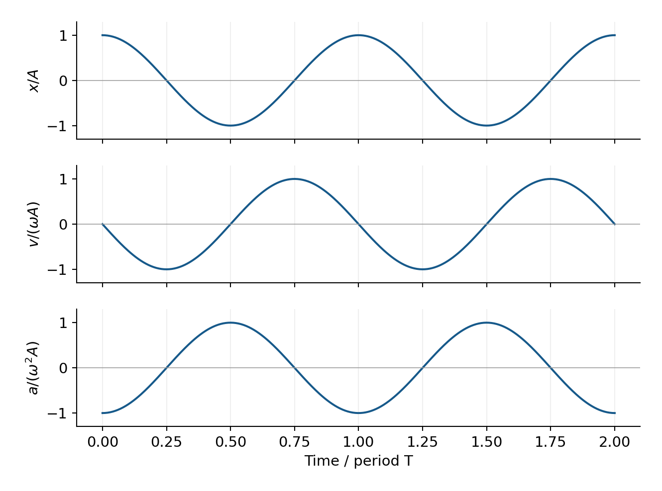
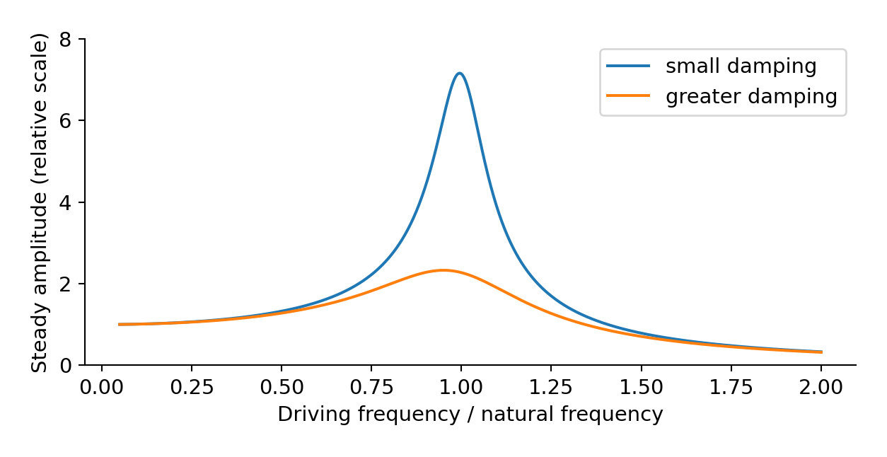
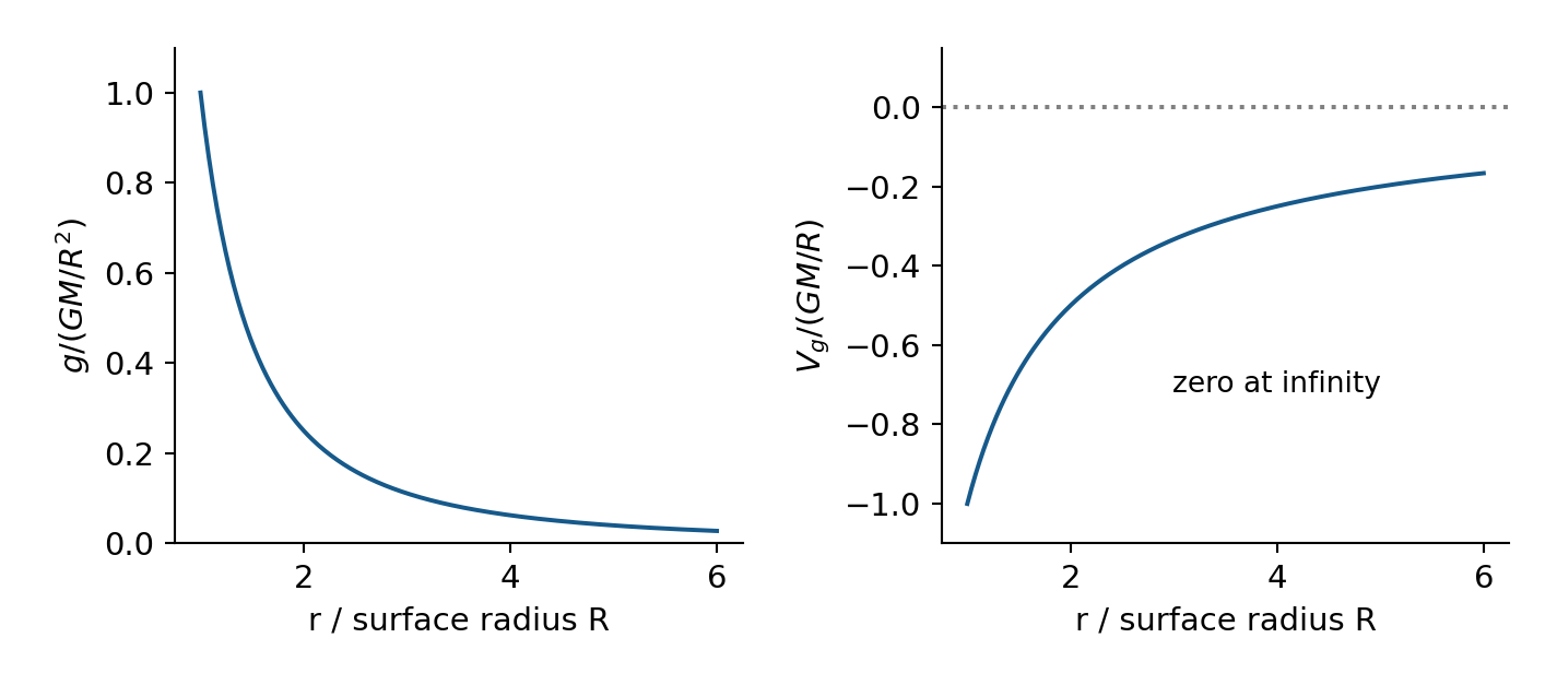
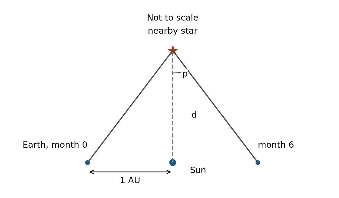
Edexcel IAL Physics Unit 1 (paper WPH11) is Mechanics and Materials 力学与材料: how things move, what forces do, how momentum and energy behave, and how solid and liquid materials respond to forces.
The paper is 1 hour 30 minutes, 80 marks, every question compulsory. It mixes multiple-choice, short answers, calculations and one or two extended-writing answers marked with an asterisk 星号 (*).
At least 32 of the 80 marks test Level-2 mathematics: reading graphs, rearranging equations, trigonometry 三角学 and areas.
A formula list is printed at the back of the paper. Learn what each symbol means and when each equation is allowed — the list gives formulas, not understanding.
Use $g = 9.81\ \text{m s}^{-2}$. The paper requires this value; using $g = 10$ can lose accuracy marks. Give final answers with a unit 单位 and a sensible number of significant figures 有效数字 (usually 2–3, matching the data).
A speedometer shows speed at one moment; a journey can still hide stops and bursts. This unit replaces one number with the full picture: graphs, vectors 矢量, forces 力, momentum 动量, energy 能量 and the strength of materials 材料.
Mechanics and Materials/mɪˈkænɪks ænd məˈtɪərɪəlz/
מכניקה וחומרים
asterisk/ˈæstərɪsk/
כוכבית
trigonometry/ˌtrɪɡəˈnɒmətri/
טריגונומטריה
unit/ˈjuːnɪt/
יחידה
significant figures/sɪɡˈnɪfɪkənt ˈfɪɡəz/
ספרות משמעותיות
vectors/ˈvektəz/
וקטורים
forces/ˈfɔːsɪz/
כוחות
momentum/məʊˈmentəm/
תנע
energy/ˈenədʒi/
אנרגיה
materials/məˈtɪərɪəlz/
חומרים
1.1
Motion: quantities and graphs
סיילבוס
יחידה 1 פיזיקה Edexcel IAL (WPH11), גרסת מפרט 3 (יולי 2021), נקודות 1–3 ו11 (מעשה ליבה 1; מספרים בין נקודות הכוח במפרט, מלמדים כאן עם תנועה).
יכול להשתמש במשוואות לתנועה באיטוצה אחידה בממד אחד: s = (u+v)t/2, v = u + at, s = ut + ½at², v² = u² + 2as
יכול לשרטט ולפרש גרפים של מקום-זמן, מהירות-זמן ותאוצה-זמן
להכיר את הגדלים הפיזיקליים הנגזרים משיפועים ושטחים של גרפים של תנועה–זמן, מהירות–זמן ותאוצה–זמן, כולל מקרים של תאוצה לא אחידה, ולהבין כיצד להשתמש בגדלים אלו
מעשה ליבה 1: קביעת התאוצה של גוף בנפילה חופשית
מקור: הסיילבוס הבינלאומי של קמבריד'ג'
English
displacement 位移 — straight-line change of position, with direction (a vector). distance 距离 — the total path length (a scalar 标量, no direction).
velocity 速度 — rate of change of displacement. speed 速率 — rate of change of distance.
acceleration 加速度 — rate of change of velocity: $a = \dfrac{\Delta v}{\Delta t}$, unit $\text{m s}^{-2}$.
Because displacement is the straight line from start to finish, a curved path always gives distance > magnitude of displacement — the examiner asks for exactly this comparison.
Reading motion graphs
On a displacement–time graph, the gradient 斜率 is the velocity. A curved line means changing velocity; take the gradient of a tangent 切线 at the point.
On a velocity–time graph, the gradient is the acceleration, and the area 面积 between the line and the time axis is the displacement. Area below the axis is negative displacement (motion backwards); distance adds the sizes of all the areas.
On an acceleration–time graph, the area under the line is the change in velocity.
Constant non-zero acceleration bends a displacement–time graph into a parabola 抛物线; a straight line on that graph means zero acceleration.
Worked example (June 2025 style). A velocity–time line rises straight from $1.8\ \text{m s}^{-1}$ at $t = 4\ \text{s}$ to $5.0\ \text{m s}^{-1}$ at $t = 16\ \text{s}$.
Known: two $(t, v)$ pairs on the straight part. Why: acceleration is the gradient of a velocity–time graph.
Check: the line rises gently, so a small acceleration is sensible.
The four suvat equations
For uniform acceleration 匀加速 (constant acceleration) in one dimension, with $s$ displacement, $u$ initial velocity, $v$ final velocity, $a$ acceleration, $t$ time:
$$v = u + at \qquad s = \frac{(u+v)t}{2} \qquad s = ut + \tfrac{1}{2}at^2 \qquad v^2 = u^2 + 2as$$
Choose the equation that contains your known quantities and the one you want — and nothing you do not know. No $t$? Use $v^2 = u^2 + 2as$. No $a$? Use $s = \tfrac{(u+v)}{2}t$.
These equations are valid only while the acceleration is constant. A curved velocity–time graph shows changing acceleration; a curved displacement–time graph can still represent constant acceleration.
Free fall is uniform acceleration with $a = g = 9.81\ \text{m s}^{-2}$ downwards (air resistance negligible 可忽略的).
Worked example (deduce-and-compare, June 2025 Q13). A basketball is thrown from $1.7\ \text{m}$ above the floor with initial vertical velocity $5.1\ \text{m s}^{-1}$ upwards, and enters the hoop moving downwards at $2.1\ \text{m s}^{-1}$. Is the hoop $3.0\ \text{m}$ above the floor?
Known: $u = +5.1\ \text{m s}^{-1}$, $v = -2.1\ \text{m s}^{-1}$ (downwards is negative), $a = -9.81\ \text{m s}^{-2}$. Wanted: the rise $\Delta s$. No time given, so use $v^2 = u^2 + 2a\Delta s$.
$$v^2 = u^2 + 2a\Delta s \quad\Rightarrow\quad \Delta s = \frac{v^2 - u^2}{2a}$$
Hoop height $= 1.7\ \text{m} + 1.1\ \text{m} = 2.8\ \text{m} \neq 3.0\ \text{m}$, so the hoop was not at the regulation height. A "deduce whether" question earns its last mark only when the comparison and conclusion are stated.
Core practical 1: measuring $g$
Drop an object and measure it: with a light gate 光电门 or video of known frame rate, get $s$ and $t$ (or velocities at two points) and use a suvat equation. Cleaner: plot $s$ against $t^2$ for $s = \tfrac{1}{2}gt^2$ — a straight line through the origin with gradient $g/2$. A straight line that misses the origin reveals a systematic offset 系统偏差, for example a fixed offset in the measured distance. A timing delay can also distort the relationship; automatic timing reduces reaction-time error. In a strobe photograph, the object moves during each flash. A shorter flash produces a sharper image and a smaller range of possible positions, reducing the uncertainty in the distance reading if the scale and image resolution are unchanged.
להבין גדלים סקלאריים ווקטוריים ולהכיר דוגמאות לכל סוג של גדל ולזהות סימון וקטורי
להיות מסוגל לפצל וקטור לשני רכיבים ניצבים זה לזה על ידי ציור ועל ידי חישוב
להיות מסוגל למצוא את הוektor הנתון (ה resultant) של שני וקטורים קו-פלנריים בכל זווית זה לזה על ידי ציור, ובניצבות זה לזה על ידי חישוב
להבין כיצד להשתמש בעצמאות התנועה האנכית והאופקית של פרוגטייל הנע בחופשיות תחת השפעת הכבידה
מקור: הסיילבוס הבינלאומי של קמבריד'ג'
English
A vector has magnitude and direction (displacement, velocity, acceleration, force, momentum); a scalar has magnitude only (distance, speed, work, energy). Vector notation in the paper is an arrow above the symbol, $\vec{F}$.
Resolving and combining
Resolving splits one vector into two perpendicular 垂直的 components: the component of force $F$ at angle $\theta$ along a direction is $F\cos\theta$ if $\theta$ is measured from that direction, $F\sin\theta$ from the perpendicular. Choose by drawing the right triangle, not by habit.
Combining two perpendicular components rebuilds the vector: magnitude $R = \sqrt{F_x^2 + F_y^2}$, direction from $\tan\theta = F_y / F_x$.
Combine before squaring. The resultant of $500\ \text{N}$ and $200\ \text{N}$ at right angles is $\sqrt{500^2 + 200^2}\ \text{N}$, not $\sqrt{500^2} + \sqrt{200^2}$.
At any angle, add vectors by drawing a scale diagram 比例图 (a vector triangle, nose to tail) or by resolving each vector into components first. In equilibrium 平衡, the vector triangle closes: $\vec{W} + \vec{T_1} + \vec{T_2} = 0$.
Worked example. A box sits on a ramp at angle $\theta$ to the horizontal, weight $W$ acting vertically down.
Why: the sliding direction is along the ramp, so resolve $W$ into components along and perpendicular to the ramp.
At constant speed the resultant force is zero, so the friction $F = W\sin\theta$ exactly. ($W\cos\theta$ acts into the ramp and is balanced by the normal contact force.)
Projectile motion
A projectile 抛体 moving freely under gravity is two independent motions: horizontal velocity constant (no horizontal force), vertical velocity changing under $g$.
The time to fall depends only on the vertical motion. Two balls leaving a table at different speeds — or with different masses — land after the same time: mass and horizontal speed do not appear in $s = ut + \tfrac{1}{2}gt^2$.
Method: resolve the launch velocity into $u_h = u\cos\theta$ and $u_v = u\sin\theta$; run suvat separately for each direction; time links the two.
Worked example (January 2025 Q19). A projectile launches at $500\ \text{m s}^{-1}$, $22^\circ$ above the horizontal, from $2.0\ \text{km}$ above the sea. Show it passes over a ship $15\ \text{km}$ away after about $30\ \text{s}$.
Known: $u$, $\theta$, horizontal distance $s_h$. Horizontal motion has $a = 0$, so use $s_h = u_h t$.
Why a maximum range exists: raising the launch angle raises $u_v$ (more time in the air) but lowers $u_h$; range $= u_h \times t$ peaks between the two effects.
Edexcel IAL Physics Unit 1 (WPH11), specification Issue 3 (July 2021), statements 8–10 and 12 (statement 11, core practical 1, is taught on sheet 1.1 with motion).
להיות מסוגל לצייר ולפרש דיאגרמות כוחות חופשיים כדי לייצג כוחות המופעלים על חלקיק או על גוף מורחב אך קשיח באמצעות מושום מרכז הכובד של גוף מורחב
יכול להשתמש במשוואה ΣF = ma, ולהבין כיצד להשתמש במשוואה זו במצבים שבהם m הוא קבוע (החוק השני של ניוטון לתנועה), כולל החוק הראשון של ניוטון לתנועה כאשר a = 0, גופים במנוחה או הנעים במהירות קבועה; שימוש במונח מהירות סופית מצופה.
להכיר ולהבין את המשוואות לעוצמת שדה כבידה g = F/m ומשקל W = mg
להכיר ולהבין את חוק תנועה השלישי של ניוטון ולהכיר את מאפי הזוגות של כוחות באינטראקציה בין שני גופים
מקור: הסיילבוס הבינלאומי של קמבריד'ג'
English
A free-body diagram 受力图 shows only the forces acting on the chosen object — never forces the object applies to other things. On an extended body, the weight acts at the centre of gravity 重心.
Newton's first law 牛顿第一定律: zero resultant force means no change in motion — at rest or moving at constant velocity. Constant velocity is not "no forces"; it is balanced forces.
Newton's second law 牛顿第二定律: $\sum F = ma$. The resultant force causes the acceleration; list every force, choose a positive direction, then apply.
Newton's third law 牛顿第三定律: when body A exerts a force on body B, B exerts an equal, opposite force on A. The pair acts on different bodies, is the same type of force, and acts along the same line. A book's weight and the table's normal contact force are not a third-law pair: they act on the same body.
weight 重量$W = mg$; gravitational field strength 重力场强度$g = \dfrac{F}{m}$, so $g = 9.81\ \text{N kg}^{-1}$.
Terminal velocity 终端速度: as a falling object speeds up, drag 阻力 grows until drag (+ upthrust) equals weight; the resultant force is then zero and the velocity stops changing. "Terminal" describes the force balance, not a speed limit printed in nature.
Worked example (June 2025 Q11). A resultant force of $4800\ \text{N}$ accelerates a boat at $0.31\ \text{m s}^{-2}$. Find the boat's weight.
Known: $\sum F$, $a$. Why: $\sum F = ma$ links them to the mass; $W = mg$ links mass to weight.
$$\sum F = ma \quad\Rightarrow\quad m = \frac{\sum F}{a} = \frac{4800\ \text{N}}{0.31\ \text{m s}^{-2}} = 15\,500\ \text{kg}$$
להכיר את עקרון שימור התנע הקווי, להבין כיצן לקשר אותו לחוקי תנועה של ניוטון ולהבין כיצד להחיל אותו על בעיות בממד אחד
מקור: הסיילבוס הבינלאומי של קמבריד'ג'
English
momentum$p = mv$, a vector, unit $\text{kg m s}^{-1}$.
Conservation of linear momentum 动量守恒: when the resultant external force is zero (or its impulse during a short interaction is negligible), total momentum before an event equals total momentum after. Give velocities signs: choose one direction as positive and keep it.
Momentum conservation follows from Newton's second and third laws: the forces between the two bodies are equal and opposite, act for the same time, so the changes of momentum are equal and opposite.
Kinetic energy need not survive a collision; momentum always does (in an isolated system 孤立系统).
Worked example (June 2025 Q10). A train of mass $3m$ at speed $v$ meets a truck of mass $m$ at speed $2v$ the other way; they couple. Find the new speed.
Known: masses, velocities in opposite directions. Why: an isolated pair, so conserve momentum with signs. Take the train's direction as positive.
$$p_{\text{before}} = p_{\text{after}}$$
$$3m \times v + m \times (-2v) = (3m + m)\,V$$
$$mv = 4mV \quad\Rightarrow\quad V = \frac{v}{4}$$
Check: the momenta nearly cancel, so a small combined speed in the train's direction is sensible.
be able to use the equation for the moment of a force, moment of force = Fx, where x is the perpendicular distance between the line of action of the force and the axis of rotation
be able to use the concept of centre of gravity of an extended body and apply the principle of moments to an extended body in equilibrium
מקור: הסיילבוס הבינלאומי של קמבריד'ג'
English
The moment of a force 力矩 about a pivot 支点 is $\text{moment} = Fx$, where $x$ is the perpendicular distance 垂直距离 from the pivot to the force's line of action. If the force meets the lever at angle $\theta$, use the perpendicular component $F\sin\theta$ or the perpendicular distance — never both.
Principle of moments 力矩原理: in equilibrium, total clockwise moment = total anticlockwise moment (resultant moment is zero).
Full equilibrium needs both: resultant force zero and resultant moment zero. A see-saw with equal children at equal distances has both; the same children at unequal distances still balance forces but not moments.
For a uniform 均匀的 beam, the weight acts at its centre.
Worked example (June 2025 Q19). A uniform rail, length $1.40\ \text{m}$, weight $95\ \text{N}$, lies at $42^\circ$ to the horizontal, pivoted at one end. A piston pushes with $160\ \text{N}$ at $18^\circ$ to the rail, $0.37\ \text{m}$ from the pivot. What perpendicular force $F$ at the handle end just lifts the rail?
Known: geometry, both forces, both angles. Why: just lifting means equilibrium at the pivot, so apply the principle of moments with perpendicular parts.
A vertical pull at the handle instead: its perpendicular distance to the pivot is shorter than the rail's length, so a larger force would be needed for the same moment.
Edexcel IAL Physics Unit 1 (WPH11), תוכנית לימודים Issue 3 (יולי 2021), סעיפים 17–22.
יכול ליישם את המשוואה לעבודה ΔW = FΔs, כולל חישובים כאשר הכוח אינו לאורך קו התנועה
יכול ליישם את המשוואה Ek = ½mv² לאנרגיה הקינטית של גוף
יכול ליישם את המשוואה ΔEgrav = mgΔh להפרש באנרגיה פוטנציאלית כבידתית בסמוך לפני שטח כדור הארץ
יודע ומבין כיצד ליישם את עיקר השימור באנרגיה, כולל שימוש בעבודה שנעשתה, אנרגיה פוטנציאלית כבידתית ואנרגיה קינטית
יכול ליישם את המשוואות הקושרות בין הספק, זמן ואנרגיה שהועברה או עבודה שנעשתה P = E/t ו-P = W/t
יכול ליישם את המשוואות יעילות = אנרגיה מועילה ביציאה / סך כל האנרגיה בכניסה ויעילות = הספק מועיל ביציאה / סך כל ההספק בכניסה
מקור: הסיילבוס הבינלאומי של קמבריד'ג'
English
work 功$\Delta W = F\Delta s$ when the force acts along the motion; if the force is at angle $\theta$ to the motion, only the component along the motion works: $\Delta W = F\Delta s\cos\theta$.
kinetic energy 动能$E_k = \tfrac{1}{2}mv^2$ — doubling speed quadruples the energy.
gravitational potential energy 重力势能$\Delta E_{\text{grav}} = mg\Delta h$ near the Earth's surface.
Conservation of energy 能量守恒: energy is transferred or transformed, never created or destroyed. In a fall with drag, $\Delta E_{\text{grav}}$ becomes $E_k$plus work done against air resistance; at terminal velocity $E_k$ is constant, so all of the $\Delta E_{\text{grav}}$ goes to work against drag.
power 功率$P = \dfrac{E}{t} = \dfrac{W}{t}$ — energy transferred per unit time.
efficiency 效率$= \dfrac{\text{useful energy output}}{\text{total energy input}} = \dfrac{\text{useful power output}}{\text{total power input}}$.
Worked example (June 2025 Q14). An electric car of $1800\ \text{kg}$ at $14\ \text{m s}^{-1}$ brakes to rest on a hill, gaining $0.76\ \text{m}$ of height; the battery gains $45\ \text{kJ}$. Find the efficiency of the braking.
Known: $m$, $v$, $\Delta h$, battery gain. Why: the total input is the energy the brakes remove — kinetic energy lost minus the gravitational energy the car keeps by ending higher.
Edexcel IAL Physics Unit 1 (WPH11), תוכנית לימודים Issue 3 (יולי 2021), סעיפים 23–26.
יכול ליישם את המשוואה צפיפות ρ = m/V
מבין כיצד להשתמש בקשר כוח הדחף = משקל הנוזל הרדוף
א) יכול ליישם את המשוואה לחיכוך ויסקוזי (חוק סטוקס) F = 6πηrv; ב) מבין שמשוואה זו חלה רק על עצמים כדוריים קטנים הנעים במהירויות נמוכות עם זרימה למינרית (או בהיעדר זרימה טורבולנטית) והוויסקוזיות תלו בטמפרטורה
ניסוי ליבה 2: שימוש בשיטת כדור נופל כדי לקבוע את הוויסקוזיות של נוזל
מקור: הסיילבוס הבינלאומי של קמבריד'ג'
English
density 密度$\rho = \dfrac{m}{V}$. For a sphere, $V = \tfrac{4}{3}\pi r^3$.
upthrust 浮力 = weight of the fluid displaced 排开的流体 — the displaced weight, not its volume or its mass.
Stokes' law 斯托克斯定律: viscous drag on a small sphere at low speed in laminar flow 层流 is $F = 6\pi\eta rv$, with $\eta$ the viscosity 黏度, $r$ the radius, $v$ the speed. It is valid only for small spheres moving slowly without turbulence 湍流, and $\eta$ falls as the liquid warms in this experiment; gases do not generally follow this trend.
Core practical 2: viscosity by the falling-ball method
Drop a ball-bearing into a measuring cylinder of the liquid. Wait until it falls at terminal velocity, then time it over a marked distance. At terminal velocity, the forces balance: weight = upthrust + drag, so
You need the ball's radius and mass (or its density), the oil's density, the fall distance and the time. Warm oil is less viscous, so the ball falls faster and the measured time is shorter.
Edexcel IAL Physics Unit 1 (WPH11), תוכנית לימודים Issue 3 (יולי 2021), סעיפים 27–32.
יכול ליישם את משוואת חוק הוק ΔF = kΔx, כאשר k הוא קשיחות הגוף
מבין כיצד להשתמש בקשרים (מתיחה או דחיסה) מתח = כוח / שטח חתך, עיוות = שינוי באורך / אורך מקורי, ומדד יאנג = מתח / עיוות
א) יכול לשרטט ולפרש גרפים של כוח-התאמה וכוח-דחיסה; ב) להבין את המונחים: גבול פרופורציונליות, גבול אלסטי, נקודת פלישה, עיוות אלסטי ועיוות פלסטי, ולהיכנס ליישוםם בגרפים אלו
יכול לשרטט ולפרש גרפי מתח-עיוות במתיחה או בדחיסה, ולהבין את מונח המתח השבר
מעבדה ליבה 3: קביעת מקדם יאנג לחומר
יכול לחשב את האנרגיה העיוותית האלסטית Eel בדוגמאת חומר מעוותת, באמצעות המשוואה ΔEel = ½FΔx, ובאמצעות השטח תחת הגרף כוח-התאמה; צפוי הערכה של שטח ולכן שינוי אנרגיה עבור גרפי כוח-התאמה ליניאריים ולא-ליניאריים
מקור: הסיילבוס הבינלאומי של קמבריד'ג'
English
Hooke's law 胡克定律: $\Delta F = k\,\Delta x$ while the material behaves proportionally; $k$ is the stiffness 刚度 (spring constant 弹簧常数), the gradient of the force–extension graph.
stress 应力$\sigma = \dfrac{F}{A}$ (unit Pa), strain 应变$\varepsilon = \dfrac{\Delta x}{x}$ (no unit), Young modulus 杨氏模量$E = \dfrac{\sigma}{\varepsilon}$. Stress and strain describe the material; force and extension describe the sample.
On a force–extension or stress–strain graph: the straight part ends at the limit of proportionality 比例极限; beyond the elastic limit 弹性极限 the sample no longer returns to its original length (elastic deformation 弹性形变 = it does return; plastic deformation 塑性形变 = it stays stretched); a material with a distinct yield point can stretch substantially with little increase in force at yield; other ductile materials yield gradually. The yield point 屈服点 marks the onset of substantial plastic flow; the breaking stress 断裂应力 is the stress at fracture.
elastic strain energy 弹性应变能: $\Delta E_{\text{el}} = \tfrac{1}{2}F\Delta x$ for a linear spring — the area under the force–extension graph. For a non-linear graph, estimate the area by squares. The area under a loading stress–strain graph is the work done per unit volume 单位体积, because $\dfrac{F}{A} \times \dfrac{\Delta x}{x} = \dfrac{F\Delta x}{V}$. In the elastic region this is stored recoverably as elastic strain energy; work beyond the elastic limit is not all recoverable.
Worked example (June 2025 Q17b). A violin string of original length $0.750\ \text{m}$ and radius $0.85 \times 10^{-3}\ \text{m}$ stretches to $0.752\ \text{m}$ under $36\ \text{N}$. Find the Young modulus.
Known: $F$, $x$, $\Delta x$, $r$. Why: $E = \sigma/\varepsilon$ needs stress and strain; stress needs the cross-sectional area.
Check: a metal-wire modulus is $10^{9}$–$10^{12}\ \text{Pa}$; $6\ \text{GPa}$ sits in range.
Core practical 3: the Young modulus of a wire
Hang known weights on a long wire and measure the extension with a marker against a scale; keep the wire long and the extensions small for precision, add loads in steps within the proportional region, and measure the diameter in several places with a micrometer 千分尺. Then $E$ comes from the gradient of the stress–strain line, or from $\sigma/\varepsilon$ point by point within the proportional region.
limit of proportionality/ˈlɪmɪt ɒv prəˌpɔːʃəˈnælɪti/
גבול פרופורציונליות
elastic limit/ɪˈlæstɪk ˈlɪmɪt/
גבול אלסטי
elastic deformation/ɪˈlæstɪk ˌdiːfɔːˈmeɪʃn/
עיוות אלסטי
plastic deformation/ˈplæstɪk ˌdiːfɔːˈmeɪʃn/
עיוות פלסטי
yield point/jiːld pɔɪnt/
נקודת זרימה
breaking stress/ˈbreɪkɪŋ stres/
מתיחת שבירה
elastic strain energy/ɪˈlæstɪk streɪn ˈenədʒi/
אנרגיית עיוות אלסטית
per unit volume/pɜː ˈjuːnɪt ˈvɒljuːm/
לכל יחידת נפח
micrometer/maɪˈkrɒmɪtə/
מיקרומטר
1.8
Exam craft for WPH11
English
Show every step. "Use of $F = ma$" earns a mark before any number appears — write the equation in symbols, then substitute.
Units and $g$. A missing unit usually loses the final mark; $g = 10\ \text{m s}^{-2}$ can lose accuracy marks; "show that" questions need one more significant figure than the target value.
Command words:state = a short precise answer; calculate/determine = numbers with working and a unit; deduce = working plus a compared conclusion; explain = linked physics reasons; describe = what happens, in order.
The asterisk (*) answer is marked for linked, logical reasoning as well as content: order the points, then link them.
The formula list is at the back — know where, so you never memorise what you can look up in two seconds.
1.8
Check yourself
English
On a velocity–time graph, what do the gradient and the area give? — acceleration; displacement.
Which suvat equation finds a height from two velocities without time? — $v^2 = u^2 + 2as$.
A projectile's horizontal acceleration in free flight? — zero (only gravity acts, vertically).
A book rests on a table: are its weight and the table's normal force a Newton's-third-law pair? — No: they act on the same body.
Two trolleys collide and stick. Which quantity is always conserved? — total momentum (kinetic energy need not be).
A force at an angle to a lever: which distance goes into the moment? — the perpendicular distance from the pivot to the line of action.
A car brakes uphill: what is the input energy for the efficiency? — the kinetic energy lost minus the gravitational energy gained.
Upthrust equals the weight of what? — the fluid displaced.
Stokes' law needs which three conditions? — small sphere, low speed, laminar flow (and $\eta$ is temperature-dependent).
On a stress–strain graph, what is the gradient of the straight part, and what is the area beneath it? — the Young modulus; the elastic strain energy per unit volume.
Pearson Edexcel IAL Physics, WPH12/01, מהדורה 3 (יולי 2021), הדפסה עמ'20–23 (PDF עמ'24–27).
העתקה נאמנה של מחזור ראשי לדרישות מסומנות; טקסט מתמטי תקן מהשכבת הטקסט של ה-PDF. זהו היקף תוכנית, לא מדריך לתלמיד.
להבין: רוחב, תדר, תקופה, מהירות ואורך גל.
להשתמש במשוואת הגלים v = fλ.
לתאר גלים אורכיים באמצעות שינוי לחץ והזזת מולקולות.
לתאר גלים רוחביים.
לשרטט ולפרש גרפים המייצגים גלים רוחביים ואורכיים, כולל גלים עומדים/מונים.
Pearson Edexcel IAL Physics, WPH12/01, מהדורה 3 (יולי 2021), הדפסה עמ'20–23 (PDF עמ'24–27).
העתקה נאמנה של מחזור ראשי לדרישות מסומנות; טקסט מתמטי תקן מהשכבת הטקסט של ה-PDF. זהו היקף תוכנית, לא מדריך לתלמיד.
מעבדה ליבה 4: קביעת מהירות הקול באוויר באמצעות אוסיiloscope-קרן ⟨2⟩, יצרן אות, רמקול ומיקרופון.
להבין: חזית גל, קוהרנטיות, הפרש מסלול, סופרפוזיציה, התערבות ופאזה.
להשתמש בקשר בין הפרש פאזה להפרש מסלול.
להבין גל עומד/מון ואופן היווצרותו; לזהות נקודות קיבוע ונקודות קיבוע מלא.
להשתמש במהירות של גל רוחבי על מיתר: v = √(T/μ).
מעבדה ליבה 5: חקירה השפעת אורך, מתח ומסה ליחידת אורך על תדר של מיתר או חוט רועד.
Pearson Edexcel IAL Physics, WPH12/01, מהדורה 3 (יולי 2021), הדפסה עמ'20–23 (PDF עמ'24–27).
העתקה נאמנה של מחזור ראשי לדרישות מסומנות; טקסט מתמטי תקן מהשכבת הטקסט של ה-PDF. זהו היקף תוכנית, לא מדריך לתלמיד.
השתמש בעוצמת קרינה I = P/A.
הבן את חוק סנל n₁ sin θ₁ = n₂ sin θ₂ בגבול, כאשר מקדם שבירה n = c/v.
חשב זווית גבול באמצעות sin C = 1/n.
נבא האם מתרחשת השתכפות פנימית מלאה בגבול.
הבן כיצד למדוד את מקדם השבירה של חומר מוצק.
הבן קיטוב מישורי.
מקור: הסיילבוס הבינלאומי של קמבריד'ג'
2.4עיכוב ופולס-אקו (טווח statements 50–56, ניסוי ליבה 6)
Pearson Edexcel IAL Physics, WPH12/01, מהדורה 3 (יולי 2021), הדפסה עמ'20–23 (PDF עמ'24–27).
העתקה נאמנה של מחזור ראשי לדרישות מסומנות; טקסט מתמטי תקן מהשכבת הטקסט של ה-PDF. זהו היקף תוכנית, לא מדריך לתלמיד.
הבן עקיפה והשתמש בבניית הויגנס כדי להסביר גלים הפוגעים בחריץ או במחסום.
השתמש בנוסחת רשת העקיפה nλ = d sin θ.
מעשה לבית-ספר CORE 6: קבע אורך גל של אור לייזר או מקור אור אחר באמצעות רשת עקיפה.
הסבר כיצד ניסויי עקיפה מספקים ראיות לטבע הגלי של אלקטרונים.
השתמש בנוסחת דה-ברולי λ = h/p.
הבן מעבר והשתכפות בגבול בין תווכים.
הבן כיצד שיטת הדחייה-החזרה ממוקמת עצם, ואת הגבולות הנגזרים מאורך גל הקרינה או ממשך הפולס.
Pearson Edexcel IAL Physics, WPH12/01, מהדורה 3 (יולי 2021), הדפסה עמ'20–23 (PDF עמ'24–27).
העתקה נאמנה של מחזור ראשי לדרישות מסומנות; טקסט מתמטי תקן מהשכבת הטקסט של ה-PDF. זהו היקף תוכנית, לא מדריך לתלמיד.
הבן קרינה אלקטרומגנטית במודל הגלי ובמודל הפוטון, וכיצד המודלים התפתחו לאורך הזמן.
השתמש בנוסחה E = hf לקשר בין אנרגיית פוטון לתדר הגל.
הבן בליעת פוטונים וגרמת שחרור אלקטרוניים (אפקט פוטואלקטרי).
להבין תדירות סף ופונקציית עבודה; להשתמש ב-hf = φ + ½mv²max.
השתמש באלקטרון-וולט (eV) עבור אנרגיות קטנות.
הסבר את ההוכחה לפוטואלקטרי על טבע החלקיקים של קרן אלקטרומגנטית.
הסבר ספקטרום קווי אטומי עם מעברים בין רמות אנרגיה בדידות; חשב תדירויות נפלטות/נספגות.
מקור: הסיילבוס הבינלאומי של קמבריד'ג'
2.6זרם, התנגדות ומעגלים (טווח statements 64–73, ניסוי ליבה 7)
Pearson Edexcel IAL Physics, WPH12/01, מהדורה 3 (יולי 2021), הדפסה עמ'20–23 (PDF עמ'24–27).
העתקה נאמנה של מחזור ראשי לדרישות מסומנות; טקסט מתמטי תקן מהשכבת הטקסט של ה-PDF. זהו היקף תוכנית, לא מדריך לתלמיד.
הבנת זרם כשיעור זרימת חלקיקים טעונים; השתמש ב-I = ΔQ/Δt.
השתמש ב-V = W/Q.
הבנת R = V/I כהגדרת התנגדות; חוק אוהם I ∝ V הוא מקרה פרטי בטמפרטורה קבועה.
הסבר חלוקת הזרם באמצעות שימור מטען וחלוקת הפרש הפוטנציאלים באמצעות שימור אנרגיה.
נגזר והשתמש במשוואות התנגדות בסדרה ובמקביל מתוך שימור מטען ואנרגיה.
להשתמש ב-P = VI וב-W = VIt; לגזור ולהשתמש ב-P = I²R וב-P = V²/R.
עבודה מעשית ליבה 7: קביעת התנגדות סגנונית של חומר.
השתמש ב-I = nqvA כדי להסביר את הטווח הרחב של התנגדות סגנונית בחומרים שונים.
מקור: הסיילבוס הבינלאומי של קמבריד'ג'
2.7מחלקת מתח, חיישנים וכוח חשמלי (טווח statements 74–80, ניסוי ליבה 8)
Pearson Edexcel IAL Physics, WPH12/01, מהדורה 3 (יולי 2021), הדפסה עמ'20–23 (PDF עמ'24–27).
העתקה נאמנה של מחזור ראשי לדרישות מסומנות; טקסט מתמטי תקן מהשכבת הטקסט של ה-PDF. זהו היקף תוכנית, לא מדריך לתלמיד.
הבנת שינוי הפוטנציאל לאורך המרחק בחוט נושא זרם אחיד.
הבנת עקרונות מחלקת מתח; חשב הפרשי פוטנציאל והתנגדויות.
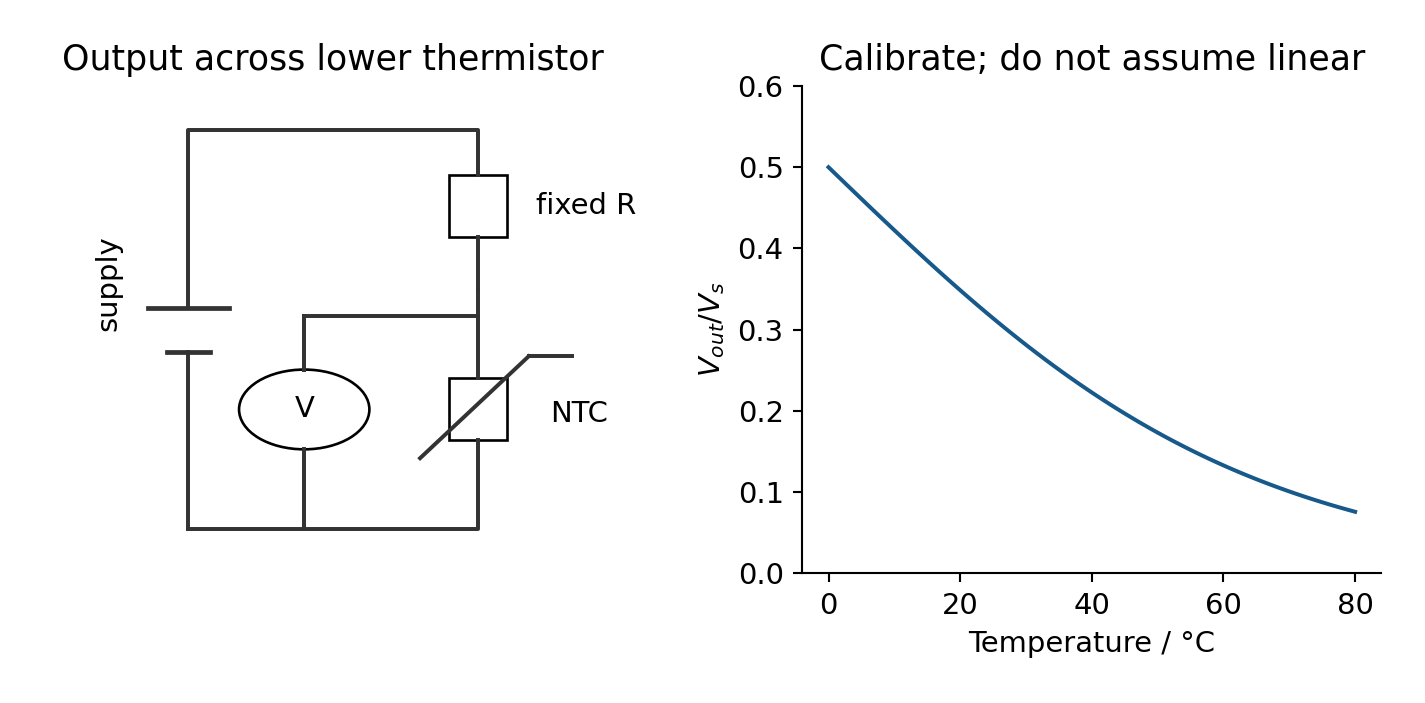
ניתוח מחלקות מתח עם התנגדות משתנה, כולל תרמיסטורים ו-LDRs.
הגדר כוח חשמלי (e.m.f.) והתנגדות פנימית; הבדל בין כוח חשמלי להפרש פוטנציאל בקצוות.
עבודה מעשית ליבה 8: קביעת כוח חשמלי והתנגדות פנימית של תא חשמלי.
דגום התנגדות תלויה בטמפרטורה באמצעות תנודות רשת ומספר אלקטרונים מוליכים; יישום לסגסוגות ולתרמיסטורים בעלי מקדם טמפרטורה שלילי.
דגם התנגדות תלויה בתאורה באמצעות מספר אלקטרונות הולכה; יישום ל-LDRs.
מקור: הסיילבוס הבינלאומי של קמבריד'ג'
חומר עזר
English
From a phone signal to its battery
Your phone receives waves and uses electrical energy. These seem different, but both depend on energy transfer. Waves 波 carry energy without carrying matter along with them. A circuit transfers energy through moving charge.
This reference covers WPH12 Waves and Electricity, specification statements 33–80. The paper lasts 90 minutes and carries 80 marks. Use the formula list to support your reasoning. Explain why an equation fits the situation, show conversions, and finish comparisons with a conclusion.
Wave quantities and graphs
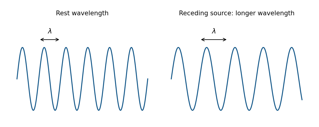
A vibrating source repeats its motion. The amplitude 振幅 is the greatest displacement from equilibrium. Equilibrium 平衡位置 means the resting position. The period 周期$T$ is the time for one complete vibration. The frequency 频率$f$ is the number of complete vibrations each second; its unit is hertz, Hz.
$$f = \frac{1}{T} \qquad v = f\lambda$$
The wavelength 波长$\lambda$ is the distance between nearest points vibrating in phase. The wave speed 波速$v$ is the speed at which a fixed phase, such as a crest, travels. It is not the speed of a vibrating particle.
A transverse wave 横波 has vibrations perpendicular to its direction of travel. A rope moves up and down while its disturbance travels along the rope.
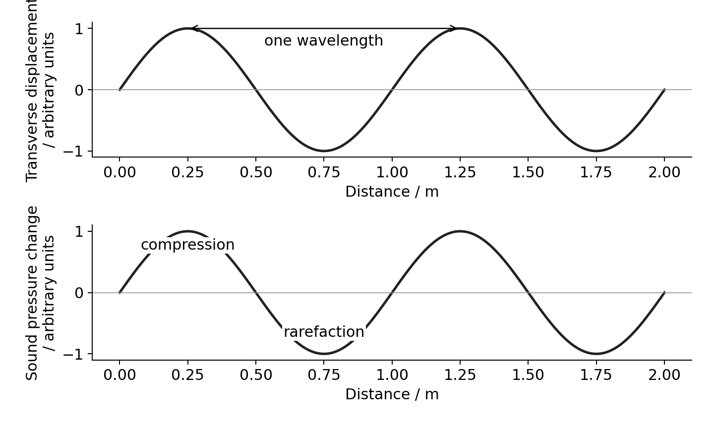
A longitudinal wave 纵波 has vibrations parallel to its direction of travel. Sound has compressions 密部, where pressure and density are higher, and rarefactions 疏部, where they are lower.
Air molecules move back and forth about their resting positions. They do not travel from the speaker to your ear with the sound.
Distance graphs show a whole wave at one instant.
Read the horizontal axis first
A displacement–distance graph is a snapshot. The separation of neighbouring crests gives $\lambda$. A displacement–time graph follows one particle. The separation of neighbouring peaks gives $T$. The same curve shape can represent either graph, but the quantities are different.
For a longitudinal wave, a pressure–distance graph shows compressions at pressure maxima. A molecular displacement–distance graph shows displacement along the direction of travel. Maximum compression occurs where displacement changes most rapidly towards the neighbouring molecules. Pressure maximum and displacement maximum are not at the same place; their patterns are one-quarter wavelength apart in a sinusoidal travelling sound wave.
Worked example. A microphone records 12 complete cycles in $0.030\ \text{s}$. Sound travels at $340\ \text{m s}^{-1}$. Find its frequency and wavelength.
Known: cycle count, total time and speed. Frequency counts cycles per second; the wave equation then links speed to wavelength.
Check: one cycle takes $T=1/f=0.0025\ \text{s}$. Twelve cycles take the stated $0.030\ \text{s}$.
Superposition and standing waves
A wavefront 波阵面 joins points at the same phase. Phase 相位 describes the stage of a vibration cycle. One complete cycle corresponds to $360^\circ$ or $2\pi$ radians.
Superposition 叠加 means adding the displacements of overlapping waves at each point. Interference 干涉 is the resulting reinforcement or cancellation. Coherent sources 相干波源 have the same frequency and a constant phase difference. Their phase difference need not be zero.
For waves of the same wavelength, the phase difference caused by a path difference 路程差$\Delta x$ is:
For sources initially in phase, path differences $0,\lambda,2\lambda,\ldots$ give constructive interference. Half-integer wavelength differences give destructive interference. Complete cancellation also needs equal amplitudes. If sources start with a phase difference, include it too.
Worked example. Two in-phase speakers produce wavelength $0.80\ \text{m}$. Their paths to a microphone differ by $1.20\ \text{m}$.
Known: path difference and wavelength. Convert path difference into cycles, then phase.
$540^\circ$ is equivalent to $180^\circ$. The waves arrive in opposite phase and interfere destructively. The sound need not become silent if the arriving amplitudes differ.
How a standing wave forms
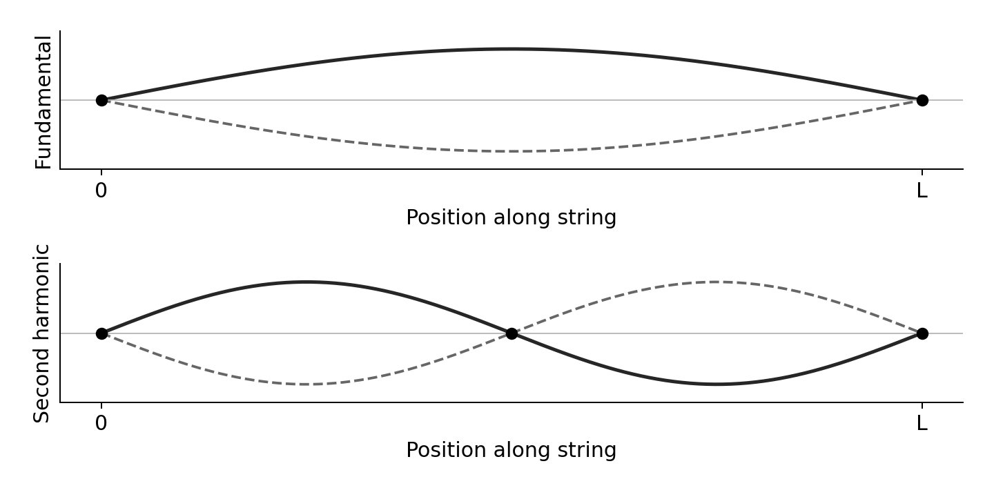
A standing wave 驻波 forms when two waves of the same frequency and similar amplitude travel in opposite directions and superpose. Reflection at a fixed string end supplies the returning wave.
A node 波节 always has zero displacement. An antinode 波腹 has the largest vibration amplitude.
Adjacent nodes are $\lambda/2$ apart. A node and its nearest antinode are $\lambda/4$ apart.
Points between the same pair of nodes vibrate in phase. Points in neighbouring sections vibrate in opposite phase.
All points have the same frequency, except that a node does not vibrate. Amplitude depends on position.
An ideal standing wave has no net energy transfer along it. A travelling wave carries energy along its direction of travel.
The end nodes remain still; the curve changes between the solid and dashed shapes.
For a string fixed at both ends, length $L$ contains a whole number $k$ of half-wavelengths:
$$L = \frac{k\lambda}{2} \qquad v = \sqrt{\frac{T}{\mu}} \qquad f = \frac{k}{2L}\sqrt{\frac{T}{\mu}}$$
Here $T$ is tension 张力, not period; $\mu$ is mass per unit length 线密度 in $\text{kg m}^{-1}$. The fundamental has $k=1$. At fixed mode, frequency increases with $\sqrt{T}$, decreases with $L$, and decreases with $\sqrt{\mu}$.
Worked example. A $0.60\ \text{m}$ string has $\mu=1.5\times10^{-3}\ \text{kg m}^{-1}$ and tension $24\ \text{N}$. Find its fundamental frequency.
Known: length, tension and linear density. The fundamental fits half a wavelength between the fixed ends.
Doubling tension multiplies frequency by $\sqrt{2}$, rather than by two.
Standing sound in a closed tube
In the simplest standing sound wave in a tube closed at one end, the closed end is a molecular displacement node. The open end is approximately a displacement antinode. This fits one-quarter wavelength into the effective tube length, so $L_{effective}=\lambda/4$. The pressure pattern is reversed: the closed end is a pressure antinode. Do not call a pressure node a displacement node. Real tubes have a small open-end correction; use an effective length if the question supplies it.
Worked example. A closed tube has effective length $0.20\ \text{m}$ and fundamental frequency $425\ \text{Hz}$. The end conditions give $\lambda=4L=0.80\ \text{m}$; then $v=f\lambda=425\times0.80=340\ \text{m s}^{-1}$. A string fixed at both ends instead fits half a wavelength in its fundamental. Choose from the end conditions, not from the word “standing”.
Core practical 4: speed of sound
Use a signal generator, speaker, movable microphone and two-beam oscilloscope 双踪示波器. Connect one oscilloscope channel to the generator reference signal and the other to the microphone output. Both traces have the same frequency.
Keep frequency constant. Move the microphone along a measured line away from the speaker. Find a position where the traces are in phase.
Move to another in-phase position. Consecutive in-phase positions are one wavelength apart. Measure across several wavelengths and divide by their number.
Read the period from the time-base scale: count horizontal divisions across several cycles, then divide. Find $f=1/T$ and use $v=f\lambda$.
Repeat positions and frequencies. Keep the microphone on the speaker axis. Reduce reflected sound by working away from walls. Measure position from a fixed microphone reference point.
Measuring several wavelengths reduces the percentage uncertainty in the distance. Measuring several periods does the same for time. A resonance-tube experiment can also measure sound speed, but it does not replace this specified practical.
Core practical 5: vibrating string
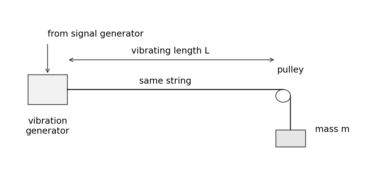
Use a vibration generator driven by a signal generator. Run the string over a pulley to a hanging mass. The tension is about $mg$ when pulley friction is small. Increase frequency until a clear standing-wave pattern forms.
Investigate tension: keep $L$, $\mu$ and mode fixed. Vary hanging mass. Plot $f^2$ against $T$; the gradient for the fundamental is $1/(4L^2\mu)$.
Investigate length: keep tension, string type and mode fixed. Plot $f$ against $1/L$.
Investigate linear density: measure string mass and length, $\mu=m/l$. Use different strings with fixed tension, vibrating length and mode. Plot $f^2$ against $1/\mu$.
Measure length between the end nodes. Find the resonance from both higher and lower frequencies and repeat. Secure the stand and keep clear of falling masses.
Intensity, refraction and polarisation
Intensity 强度 is power per unit area perpendicular to the energy flow:
$$I = \frac{P}{A}$$
Its unit is $\text{W m}^{-2}$. For a receiver, incident power is $P=IA$. Useful output is smaller if efficiency is below 100%. Convert area carefully: $1\ \text{cm}^2=10^{-4}\ \text{m}^2$.
Worked example. Radiation intensity is $800\ \text{W m}^{-2}$ over a $25\ \text{cm}^2$ solar cell. Efficiency is 20%. Can it supply $0.50\ \text{W}$?
Known: intensity, area, efficiency. First find incident power, then useful power.
$0.40\ \text{W}<0.50\ \text{W}$, so it cannot supply the required useful power.
Refraction and total internal reflection
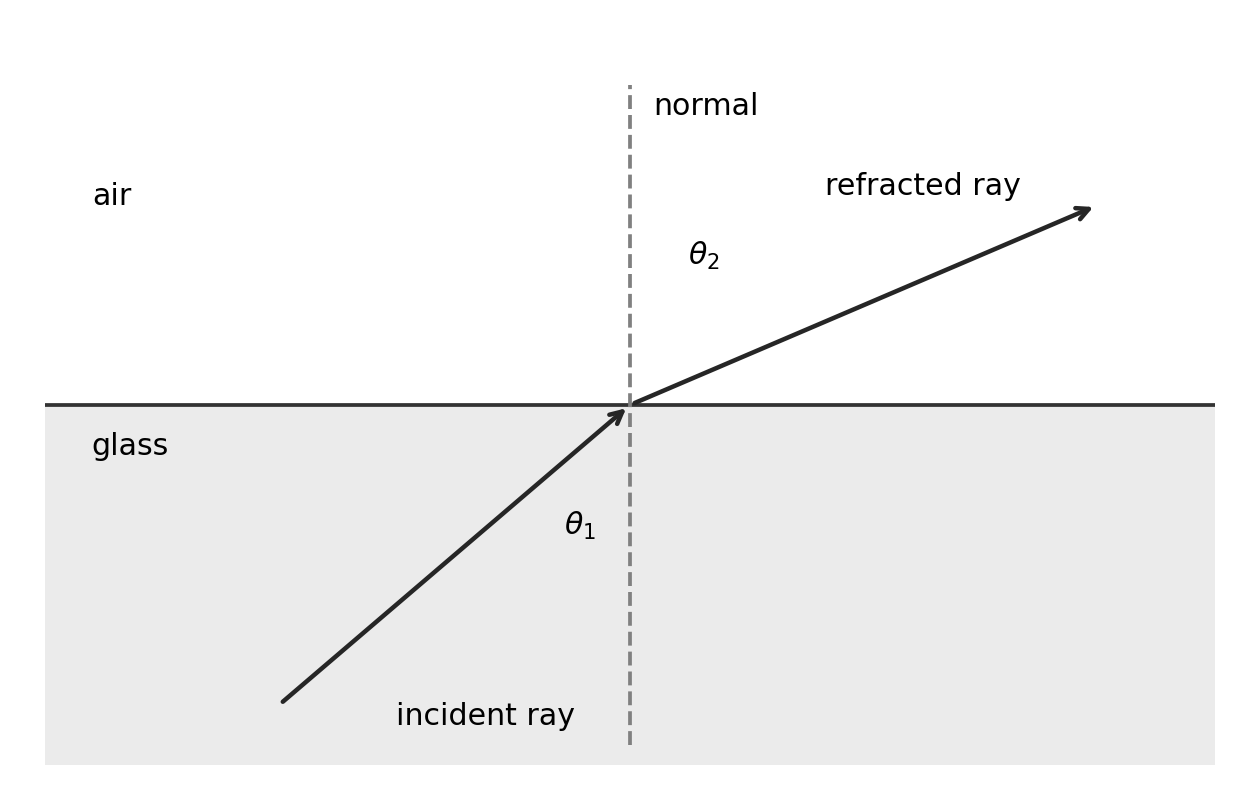
Refraction 折射 is a change in wave direction when speed changes at an interface. A ray entering along the normal changes speed without changing direction. The normal 法线 is perpendicular to the boundary. Measure all ray angles from it.
The refractive index 折射率$n$ compares vacuum light speed $c$ with speed in the material. Frequency stays constant across the boundary, so wavelength changes with speed. Entering higher $n$ bends the ray towards the normal; entering lower $n$ bends it away.
The ray bends away from the normal when it enters the lower-index medium.
Total internal reflection 全反射 requires travel from higher to lower refractive index and incidence greater than the critical angle 临界角$C$.
$$\sin C = \frac{n_2}{n_1} \qquad \text{for material to air: }\sin C = \frac{1}{n}$$
At $C$ the refracted angle is $90^\circ$; call incidence greater than $C$ total internal reflection. Below $C$, some energy is normally reflected and some transmitted. An optical fibre uses a higher-index core and lower-index cladding. Raising the cladding index raises the critical angle and can stop a previously reflected ray being trapped.
Worked example. Light travels from glass of index 1.50 into air. Does an incidence angle of $45^\circ$ produce total internal reflection?
Known: the two indices and incidence angle. Find the boundary angle before comparing.
The light travels towards lower index and $45^\circ>41.8^\circ$. Both conditions hold, so total internal reflection occurs.
Measuring refractive index
Place a rectangular transparent block on paper and trace its outline. Use a narrow ray-box beam. Mark two points on the incident ray and two on the emerging ray. Remove the block and join the boundary points to reconstruct the ray inside. Draw the normal at entry and measure incidence $i$ and refraction $r$ with a protractor.
Repeat for several incidence angles, keeping the same material and light colour. Plot $\sin i$ vertically against $\sin r$ horizontally. For air into the block, the gradient is the block's refractive index relative to air. Use a large triangle on a best-fit line. Narrow beams and widely separated ray marks reduce direction uncertainty. Very small angles give large percentage angle uncertainties.
Plane polarisation
Plane polarisation 平面偏振 restricts transverse vibrations to one plane containing the propagation direction. Unpolarised light has vibrations in many planes. A polariser transmits one vibration direction. Rotate a second polariser: parallel transmission directions give maximum brightness; perpendicular directions ideally give darkness. The ray still travels forward; its vibration direction changes selection.
Longitudinal waves cannot be plane polarised because their vibration is already along propagation. Polarisation is therefore evidence that light is transverse.
Diffraction and pulse-echo
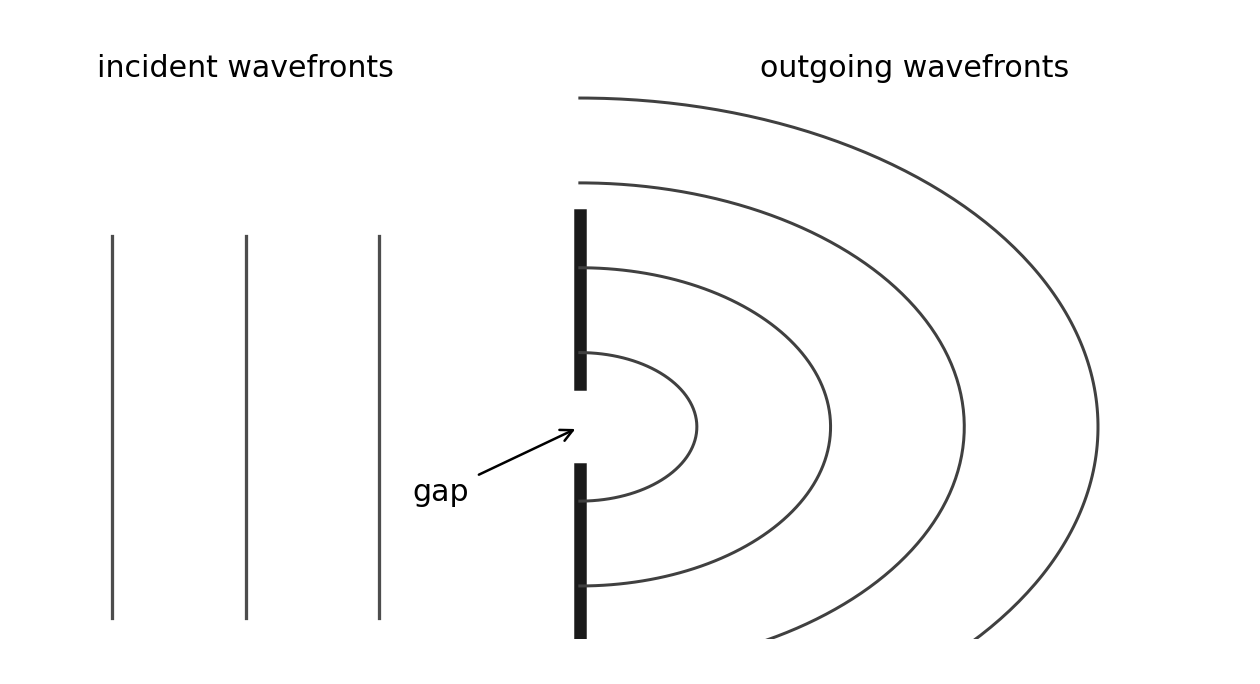
Diffraction 衍射 is the spreading of waves at a gap or edge. Spreading is greater when the gap width is comparable to the wavelength. A wide gap still diffracts at its edges, but the central wave spreads less.
In Huygens' construction 惠更斯作图法, each point on a wavefront acts as a source of secondary wavelets. Draw wavelets of equal radius after the same time. Their forward common tangent gives the new wavefront. At a narrow gap only a small part of the original front supplies wavelets, so the emerging fronts spread widely. This explains spreading without inventing a change of frequency at the slit.
The gap limits which points supply the outgoing wavelets.
Gratings and core practical 6
A diffraction grating 衍射光栅 contains many equally spaced slits. Bright maxima occur when contributions from neighbouring slits arrive in phase:
$$k\lambda = d\sin\theta$$
Here $k$ is the integer order 级次, $d$ is slit spacing, and $\theta$ is measured from the straight-through direction. The equation assumes normal incidence. If the grating has $N$ lines per metre, $d=1/N$. Do not confuse grating order with refractive index; printed papers may use $n$ for either.
Worked example. A grating has 600 lines per millimetre. First-order light appears at $18.0^\circ$. Find its wavelength.
Known: line density and first-order angle. Convert line density before taking its reciprocal.
This is $515\ \text{nm}$. Check each proposed higher order using $k\lambda/d\leq1$.
For CP6, aim a low-power laser normally at a grating and place a screen perpendicular to the central beam. Measure screen distance $D$ and displacement $x$ from the central spot to an order. Use $\tan\theta=x/D$, then the grating equation. Average corresponding left/right displacements, repeat distances, and use higher visible orders where measurement is clear. Measure from the grating to the screen, not from the laser casing. Do not substitute $\sin\theta=x/D$ unless a justified small-angle approximation is acceptable. Never look into the beam; keep it below eye level and stop stray beams.
Electrons also show wave behaviour
An electron beam passing through a thin crystal produces a diffraction pattern. Regular atom spacing provides the diffracting structure. Changing electron momentum changes the pattern spacing. This is evidence of wave behaviour; particles travelling along simple straight paths alone cannot explain the diffraction maxima.
The de Broglie wavelength 德布罗意波长 is:
$$\lambda = \frac{h}{p}$$
For a non-relativistic electron, $p=mv$. If it gains kinetic energy by crossing a potential difference, $E_k=eV$ and $p=\sqrt{2mE_k}$. Use these links only when the question gives or requires that energy relation.
Worked example. An electron has momentum $2.0\times10^{-24}\ \text{kg m s}^{-1}$. With $h=6.63\times10^{-34}\ \text{J s}$:
Increasing momentum reduces wavelength. Electrons have both particle and wave properties; diffraction does not mean that an electron becomes a sound wave.
Reflection, transmission and echoes
At an interface, part of a wave's energy may be transmitted 透射 and part reflected. A reflected pulse can locate a boundary. In pulse-echo 脉冲回波, measured delay includes the outward and return journeys:
$$2s = vt \quad\Rightarrow\quad s = \frac{vt}{2}$$
Worked example. Ultrasound travels in metal at $5900\ \text{m s}^{-1}$. An echo returns after $12\ \mu\text{s}$.
The boundary is $35\ \text{mm}$ away, not $71\ \text{mm}$. A nearby echo may overlap the transmitted pulse. Shorter pulse duration reduces this blind region and separates close echoes. Shorter wavelength helps detect or distinguish smaller features. These are related limits, but pulse duration and wavelength are not the same quantity. Use the speed in the actual material, not automatically the speed in air.
Photons and the photoelectric effect
Wave ideas explain interference, diffraction and polarisation. They did not explain all observations of energy transfer. Photons 光子 describe discrete packets of electromagnetic energy:
$$E = hf = \frac{hc}{\lambda}$$
Historically, interference and diffraction supported wave models of light. Quantum ideas developed to explain observations including the photoelectric effect and atomic spectra. Modern physics uses both wave and photon descriptions according to the measurement. A successful new model must explain evidence that the older model explains too.
One photon and one electron
In the photoelectric effect 光电效应, a surface electron absorbs a photon and may escape. The work function 逸出功$\phi$ is the minimum energy needed to remove an electron from the surface. The threshold frequency 极限频率 is $f_0=\phi/h$.
Below threshold, increasing intensity does not cause emission in the usual single-photon model.
Above threshold, higher frequency raises maximum kinetic energy. A graph of $E_{k,\max}$ against $f$ has gradient $h$, frequency intercept $f_0$ and extrapolated energy intercept $-\phi$.
At fixed frequency above threshold, higher intensity supplies more photons per second. More electrons can be emitted per second, so the saturation photocurrent rises. Their maximum kinetic energy does not rise.
Emission starts without the energy-building delay predicted by a simple continuous-wave energy model, even at low intensity above threshold.
Electrons escape with a range of kinetic energies. Some lose more energy within the material. The equation describes the largest energy, not every electron's energy.
The electronvolt 电子伏特 is an energy unit: $1\ \text{eV}=1.60\times10^{-19}\ \text{J}$. It is not a unit of potential difference. A stopping potential $V_s$ just prevents even the fastest photoelectrons reaching the collector, so $eV_s=E_{k,\max}$.
Worked example. Light of frequency $8.0\times10^{14}\ \text{Hz}$ reaches a surface with work function $2.0\ \text{eV}$.
Known: photon frequency and work function. Convert the work function into joules before subtracting.
The positive kinetic energy confirms that this frequency is above threshold. A negative subtraction would mean no emission, not negative kinetic energy.
Atomic line spectra
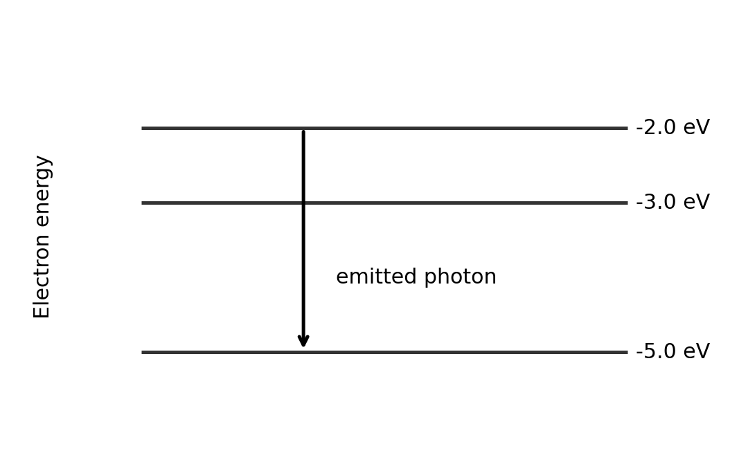
Atoms have discrete energy levels 分立能级. An electron moving down between two allowed levels emits a photon. Moving up requires absorption of the matching energy:
$$|\Delta E| = hf = \frac{hc}{\lambda}$$
A line spectrum has particular frequencies because only certain level differences are allowed. The largest downward energy difference gives the highest frequency and shortest wavelength. Count possible transitions by checking level pairs and which upper levels are populated; do not automatically count the number of levels as the number of lines.
The photon energy equals the difference between the two levels.
Worked example. An electron drops from $-2.0\ \text{eV}$ to $-5.0\ \text{eV}$.
Photon absorption in a material does not always eject an electron from its surface. Excitation followed by emission, for example in a light-activated material, is not automatically the photoelectric effect.
Current, resistance and circuits
Current 电流 is the rate of charge flow. Conventional current follows the direction positive charges would move. In a metal, electrons drift in the opposite direction.
$$I = \frac{\Delta Q}{\Delta t} \qquad V = \frac{W}{Q} \qquad R = \frac{V}{I}$$
One ampere is one coulomb per second. Potential difference 电势差$V$ is energy transferred per unit charge between two points. Resistance $R$ is defined by the ratio $V/I$ at an operating point. Ohm's law 欧姆定律 is the extra condition $I\propto V$ when temperature and other physical conditions stay constant. Not every resistor or component obeys it.
Worked example. A current of $0.40\ \text{A}$ flows for $30\ \text{s}$. Find the number of electrons passing a point.
$$Q = It = 0.40\ \text{A}\times30\ \text{s} = 12\ \text{C}$$
Charge conservation 电荷守恒 means charge does not build up at a steady-current junction. Total current entering equals total current leaving. Current is not used up by a resistor.
Energy conservation 能量守恒 means the total energy supplied per coulomb around a complete loop equals the energy transferred per coulomb. The sum of voltage rises equals the sum of voltage drops.
For series resistors, the same current passes through each and their potential differences add:
A parallel combination has smaller resistance than its smallest branch resistance. A voltmeter connects in parallel across a component; an ideal voltmeter has infinite resistance. An ammeter connects in series; an ideal ammeter has zero resistance.
Worked example. A $6.0\ \Omega$ resistor is parallel to $3.0\ \Omega$. The combination is in series with $4.0\ \Omega$ across $12\ \text{V}$.
Known: circuit arrangement. Reduce the parallel section first, then apply the series rule.
Check: branch currents add to $2.0\ \text{A}$. The remaining series resistor has an $8.0\ \text{V}$ drop.
Power and component graphs
Electrical power 电功率 is energy transferred each second. Substituting $V=IR$ into $P=VI$ gives the other forms:
$$P = VI = I^2R = \frac{V^2}{R} \qquad W = Pt = VIt$$
Use voltage across, and current through, the same component. The resistance forms apply to its operating-point resistance; do not assume a heating lamp has constant resistance.
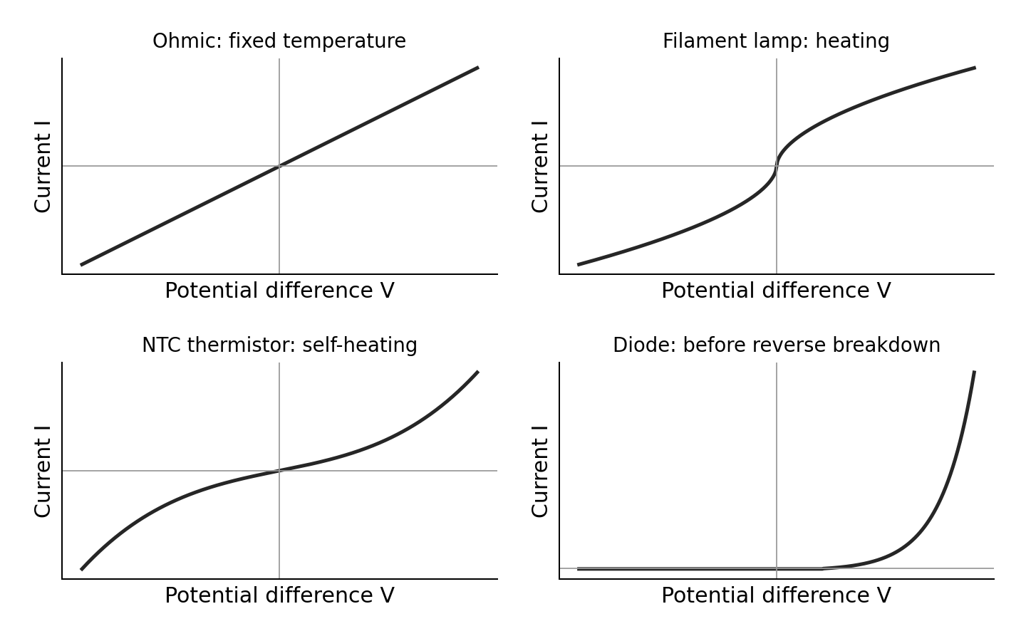
Axes and temperature conditions matter when interpreting these schematic curves.
Ohmic conductor at constant temperature: straight line through the origin. On an $I$-vertical, $V$-horizontal graph its gradient is $1/R$.
Filament lamp: as voltage magnitude rises, heating increases resistance. The $I$–$V$ curve becomes less steep.
NTC thermistor: heating lowers resistance. If current heats it sufficiently, the curve becomes steeper. At a controlled fixed temperature its behaviour over a suitable range can be approximately ohmic. Do not claim every thermistor curve must bend under every measurement condition.
Diode: very small reverse current before breakdown; forward current rises rapidly after a characteristic knee. It conducts mainly in one direction. A real diode does not have one constant resistance.
For a curved graph, $R=V/I$ uses a line from the origin to the operating point. The tangent gradient is not generally $1/R$.
Resistivity and core practical 7
Resistivity 电阻率$\rho$ is a material property at a stated temperature:
$$R = \frac{\rho l}{A} \qquad A = \frac{\pi d^2}{4}$$
Lengthening a uniform wire increases resistance. Increasing cross-sectional area decreases it. Doubling diameter gives four times the area and one-quarter the resistance, if material, length and temperature stay unchanged.
For CP7, connect a uniform wire, ammeter, power supply, switch and current-limiting resistor in series. Connect a voltmeter across the measured wire length. Measure several lengths and find $R=V/I$ for each. Plot $R$ against $l$: gradient $=\rho/A$, so $\rho=A\times\text{gradient}$.
Measure diameter with a micrometer at several positions and orientations; check its zero. Measure length between the actual electrical contacts. Use a small current and switch off between readings to limit heating. Keep contacts secure. A non-zero intercept may indicate contact or lead resistance. Repeating readings reduces scatter but does not remove a diameter zero error. Because area depends on $d^2$, a small percentage diameter uncertainty contributes about twice that percentage to area uncertainty.
Worked example. A wire diameter is $0.40\ \text{mm}$. An $R$–$l$ graph has gradient $3.5\ \Omega\,\text{m}^{-1}$.
The drift velocity 漂移速度$v$ is the small mean directed velocity of charge carriers, not their random thermal speed:
$$I = nqvA$$
Here $n$ is the number of mobile carriers per unit volume, $q$ is charge magnitude per carrier, and $A$ is cross-sectional area. A larger carrier density allows the same current with a smaller drift speed. In series wires the current is the same; changing $n$ or $A$ changes $v$.
Materials have different resistivities because their carrier densities and the ease of carrier motion differ. More scattering reduces drift speed for the same applied potential gradient. Carrier density alone does not explain every difference between materials.
Potential dividers, sensors and cells
Along a uniform wire carrying steady current at constant temperature, resistance grows in proportion to distance. The potential drop therefore grows in proportion to distance too. A potential–distance graph is straight. This assumes uniform material and area; a tapered or unevenly heated wire need not give a straight line.
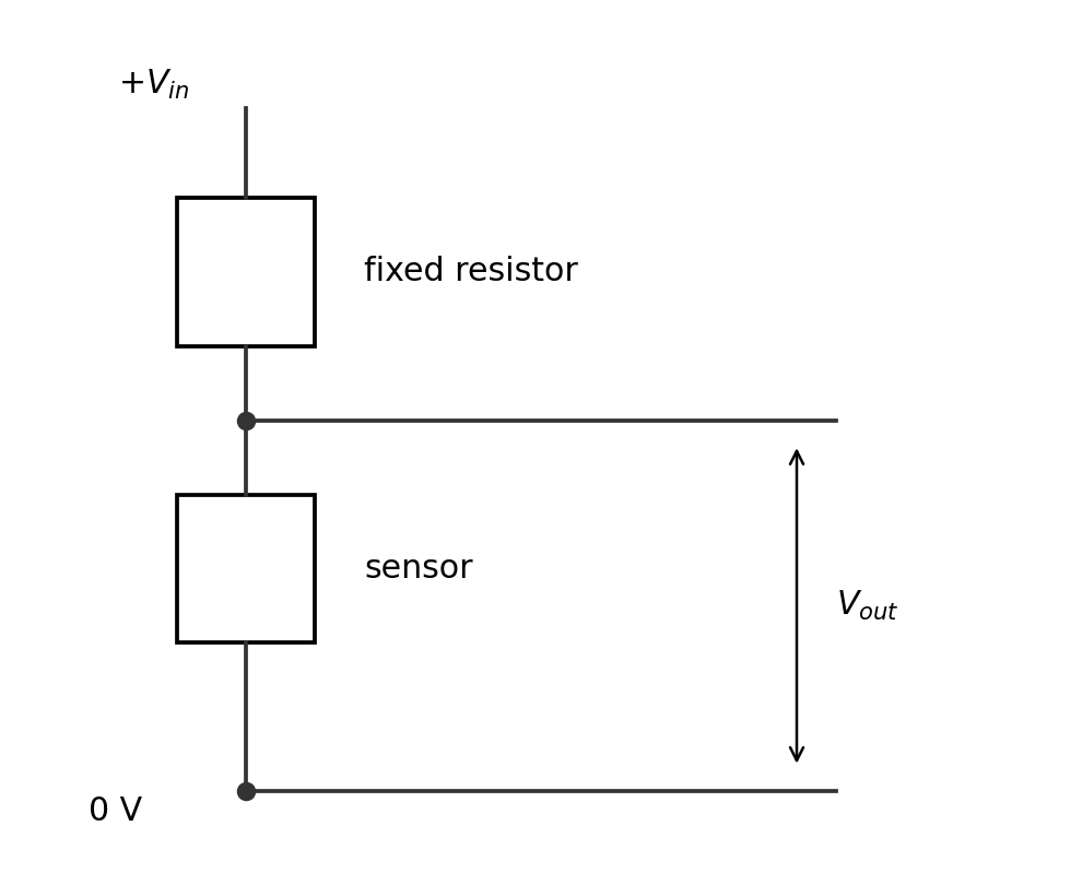
A potential divider 分压器 uses series resistances to share a supply voltage:
The expression assumes the output is unloaded, or the attached load draws negligible current. If a load draws significant current, combine it in parallel with the output resistor first. Always identify which resistor the voltmeter spans.
Swapping the sensor and fixed resistor reverses the direction of the output change.
Worked example. A $6.0\ \text{V}$ supply feeds a $2.0\ \text{k}\Omega$ fixed resistor above an LDR. Find the output across the LDR when its resistance changes from $4.0$ to $1.0\ \text{k}\Omega$.
The output across this LDR falls when illumination rises. The output across the fixed resistor rises. Explain the named output, not just “the voltage changes”.
Explain sensors using carriers
In a metal, heating increases lattice vibrations. Conduction electrons scatter more often. The mobile electron number stays approximately constant, but drift speed at a given potential gradient decreases, so resistance rises.
In a negative-temperature-coefficient thermistor 负温度系数热敏电阻, heating releases more mobile carriers. The carrier-density increase dominates, so resistance falls. Avoid saying heating reduces lattice vibrations.
In a light-dependent resistor 光敏电阻 (LDR), absorbed light releases additional mobile carriers. Increased illumination raises carrier density and lowers resistance. It does not need to work by electrons leaving its surface.
For linked explanations, give the full chain: environmental change → carrier/scattering change → resistance change → divider fraction change → named output change. Keep the circuit arrangement in view throughout.
E.m.f., internal resistance and core practical 8
Electromotive force 电动势$\mathcal{E}$ is energy supplied by the source per unit charge. It is measured in volts, despite its name. Internal resistance 内阻$r$ causes energy transfer within the source when current flows. The terminal p.d. is the energy per coulomb available to the external circuit:
$$\mathcal{E} = V+Ir \qquad V = \mathcal{E}-Ir \qquad I = \frac{\mathcal{E}}{R+r}$$
The source supplies power $\mathcal{E}I$, the external circuit receives $VI$, and internal heating is $I^2r$. These add consistently. With negligible current, terminal p.d. approaches e.m.f.
For CP8, connect a cell, ammeter, variable load and switch in series. Connect a high-resistance voltmeter across the cell terminals. Vary the external resistance and record pairs of $V$ and $I$. Plot $V$ vertically against $I$ horizontally. The best-fit line has intercept $\mathcal{E}$ and gradient $-r$. Take the magnitude of the gradient for $r$.
Use several settings and repeat. Open the switch between readings, avoid very small load resistance, and keep the cell temperature and charge state as steady as possible. Never short-circuit the cell. A graph that curves may show changing internal resistance or e.m.f.; do not force one fixed $r$ onto it without discussing the limitation.
Worked example. A cell graph passes through $(0.20\ \text{A},1.40\ \text{V})$ and $(0.60\ \text{A},1.20\ \text{V})$.
Known: two points on the best-fit line. The gradient of $V=\mathcal{E}-Ir$ is $-r$.
Check using the second point: $1.20+0.60\times0.50=1.50\ \text{V}$ too. The terminal p.d. falls as current rises.
Check yourself
Use the matching exercise sheet after each section: 2.1 wave graphs; 2.2 standing waves; 2.3 refraction; 2.4 diffraction; 2.5 photons; 2.6 circuits; 2.7 dividers and cells.
Before using a past-paper set, check that you can:
read an axis and identify whether it gives wavelength, period, pressure or displacement;
explain a practical with apparatus, measurements, controlled variables, graph and precautions;
distinguish phase from amplitude, and photon frequency from photon arrival rate;
derive circuit combinations from charge and energy conservation;
explain a sensor circuit as a connected causal chain;
use an actual comparison to finish “deduce whether”, with units and a clear conclusion.
The reviewed January and June 2025 papers supply authentic examples, but do not test every requirement. Original practice fills the teaching gaps. Completing a sampled paper alone does not prove full syllabus coverage.
Pearson Edexcel IAL Physics Issue 3 (יולי 2021), הדפסה עמ'24–26 וא Appendix 10 עמ'75–77. אלו חלוקות לימוד מקומיות, אינן הצהרות מפרט רשמית וממוספרת.
תכנן ניסוי: בחר ציוד וטווח/רזולוציה מתאימים; דן בקליברציה ובבדיקות אפס; תאר טכניקות מדידה נכונות; זיהה ושלוט במשתנים רלוונטיים נוספים; הערך האם קריאות חוזרות מתאימות; זיהה בעיות בריאות/בטיחות ושיקולים מעשיים; הסבר עיבוד נתונים; זיהה סטיות/שגיאות מערכת ודרכים להקטנתן או ביטולן; דן יתרונות/סיכונים והקשר חברתי, סביבתי או היסטורי.
מקור: הסיילבוס הבינלאומי של קמבריד'ג'
3.2מדידה, רישום ואי-ודאות
Pearson Edexcel IAL Physics Issue 3 (יולי 2021), הדפסה עמ'24–26 וא Appendix 10 עמ'75–77. אלו חלוקות לימוד מקומיות, אינן הצהרות מפרט רשמית וממוספרת.
יישום ומדידות: הערך את מספר וטווח הקריאות; רשום ספרות משמעותיות בהתאמה לרזולוציה; בדוק קריאות לא עקביות במקום למחוקן בשתיקה; קרא מכשירים, כולל מחוג מדויק (0.1 מ"מ) ומיקרומטר (0.01 מ"מ); הצע ציוד או טכניקות נוספות ספציפיים לשפר המדידה. קבע שגיאה אחוזית לקריאה יחידה באמצעות חצי הרזולוציה של המכשיר, ושגיאת קריאות חוזרות באמצעות חצי הטווח. יישם את המשמעויות ב-Appendix 10 עבור דיוק, דיוקיות, תקינות, חזרה, תקפות, שגיאה, אי-ודאות ורזולוציה.
מקור: הסיילבוס הבינלאומי של קמבריד'ג'
3.3גרפים, עיבוד נתונים ומסקנות מוצדקות
Pearson Edexcel IAL Physics Issue 3 (יולי 2021), הדפסה עמ'24–26 וא Appendix 10 עמ'75–77. אלו חלוקות לימוד מקומיות, אינן הצהרות מפרט רשמית וממוספרת.
עיבוד תוצאות: חשב עם ספרות משמעותיות ויחידות מתאימות; בחר צירי גרף/קנה מידה ועלה נתונים; פרש את הקשר וגזור קבוע מהגרף באמצעות משולש שיפוע גדול; הצע שיפורים ריאליים; דן אי-ודאות באופן איכותי/כמותי; השוו מרווח שנמדד לערך מוצע/מקובל. יחידה 3 אינה דורשת הרכבת אי-ודאויות אחוזיות. בחר טווח מתאים ונתונים נוספים ממוקדים סמוך למקסימום כאשר הדרישה דורשת זאת.
מקור: הסיילבוס הבינלאומי של קמבריד'ג'
חומר עזר
English
A number needs a method
Two groups measure the same wire. Their values differ. Which should you trust? You need more than the final number: the instrument, method, repeated readings and uncertainty all matter.
WPH13 Practical Skills in Physics I is a written paper about practical work from Units 1–2. It lasts 80 minutes and has 50 marks. All questions are compulsory. At least 20 marks assess mathematics at Level 2 or above. This guide supports real laboratory work; reading it does not replace making measurements yourself.
The three skill sheets follow the process: plan a valid investigation, collect and record measurements, then process results and justify conclusions. The official specification gives skill lists rather than numbered knowledge statements for this unit.
Planning a valid investigation
A valid measurement 有效测量 measures what you intend to measure. A precise timer does not help if it times the wrong event.
Start by naming the independent variable 自变量 that you change and the dependent variable 因变量 that you measure. List control variables 控制变量 that could also affect the dependent variable. Say how you will keep each important one steady.
Turn a description into a usable method
A method needs:
named apparatus, with a suitable measuring range and resolution 分辨率;
an arrangement showing where measurements are taken;
steps that another student can follow, including the start and end events;
several independent-variable settings over a useful range;
repeats where they test stability and estimate variation;
a calculation or graph that answers the investigation question;
specific sources of uncertainty and improvements;
realistic hazards with a practical way to reduce each risk.
Do not write only “take readings” or “use better equipment”. Name the reading, the instrument and what the improvement changes.
Worked planning example: string frequency and tension
Investigate how fundamental frequency depends on tension in a string.
Use a vibration generator and signal generator. Pass the string over a pulley to a mass hanger.
Change hanging mass $m$. With a freely moving pulley, tension is approximately $T=mg$.
Measure vibrating length between the end nodes. Use the same string and keep that length fixed.
Adjust frequency for the fundamental each time. The same mode is a control, not an optional detail.
Measure the string's mass and total length to find linear density $\mu$. Keep it unchanged in this investigation.
Record several tensions and their resonant frequencies. Repeat the tuning near each resonance.
A graph of $f^2$ vertically against $T$ horizontally should be straight through the origin. A large triangle gives the gradient. Secure the stand and keep your feet away from falling masses. This is stronger than saying “be careful”.
Calibration and zero checks
Calibration 校准 checks an instrument against known reference values. A zero error 零点误差 occurs when it does not read zero at the correct zero condition. Check closed micrometer jaws or an empty balance before measuring.
If a micrometer reads $+0.03\ \text{mm}$ with its jaws correctly closed, subtract $0.03\ \text{mm}$ from each subsequent reading. Repeating the measurement alone does not remove that offset. A zero check cannot prove that every point on the scale is calibrated correctly.
Range, spacing and repeats
Choose a range wide enough to reveal the relationship. Several measurements crowded near one setting may give a poor gradient. Use more settings near a turning point if you need to locate a maximum accurately.
Repeats are useful when conditions can be reproduced. They show scatter and help identify unstable readings. However, repeated readings of a discharging cell or a heating wire may drift because the conditions change. Reduce the current, switch off between readings, control temperature or restore conditions. Do not average a drift as though it were random variation.
Control the actual cause
When varying the angle of a lamp above a solar cell, keep lamp–cell distance and lamp output fixed. Control background light, for example with shielding or a darkened room. Keep the cell and its load the same. Otherwise a change in measured power may come from distance, illumination or circuit resistance instead of angle.
Discuss context using a physical cause. A tracking solar panel can stay closer to normal incidence and collect more energy over a day. Its motor also uses energy and adds cost or maintenance. “Better for the environment” alone does not explain either effect.
Measuring and recording
Accuracy 准确度 describes closeness to the true value. Precision 精密度 describes how closely repeated values cluster. Closely clustered results can still all share a systematic offset.
Repeatability 重复性 concerns similar results using the same operator and method over a short time.
Reproducibility 再现性 concerns similar results from different operators, apparatus or methods.
Random effects 随机影响 cause unpredictable variation. Repeating and taking a mean can reduce their influence.
Systematic error 系统误差 shifts results in a consistent way. Correct the cause or known offset; repeating does not remove it.
Uncertainty 不确定度 is a reasonable interval associated with a measurement. It is not automatically a mistake or the known size of the error.
Read instruments at their resolution
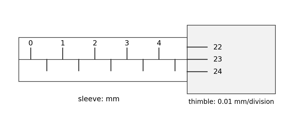
A millimetre ruler has a smallest interval of $1\ \text{mm}$. The specification's standard Vernier calipers resolve $0.1\ \text{mm}$, and its standard micrometer resolves $0.01\ \text{mm}$. Check the instrument shown: a digital display or a different scale may have a different resolution.
For a micrometer, add the visible sleeve reading and the thimble reading. Include a visible half-millimetre sleeve mark when appropriate. Use the ratchet for consistent contact pressure, rather than overtightening the jaws.
For Vernier calipers, read the main scale just before the Vernier zero, then add the aligned Vernier division times its resolution. Check that the jaws contact the intended surfaces without tilting. Do not infer a missing scale from an extracted text description: read the instrument diagram itself.
Read the sleeve before adding the aligned thimble division.
Worked example. The last visible sleeve mark is $4.5\ \text{mm}$. Thimble division 23 aligns with the reference line. Resolution is $0.01\ \text{mm}$ and zero error is $+0.02\ \text{mm}$.
Avoid parallax 视差 by viewing a scale along the correct line of sight. Use a set square to transfer a height or position onto a ruler. Keep the ruler parallel to the distance being measured; a sloping ruler measures a different distance.
A light gate measures the blocking time of an interrupting object. With known interrupting length $l$, speed is $v=l/t$. That gives speed during passage, not acceleration by itself. To find acceleration, measure a change of speed over known time, or use a justified motion equation with additional measured quantities. Do not call $l/t$ acceleration.
A video with known frame rate can reduce reaction-time uncertainty. Count frames between clearly defined start and end events, then use $t=N/f_{\text{frame}}$. The frame interval limits timing resolution. Blurred images or unclear event positions can still limit the result.
Tables and significant figures
Put quantity and unit together in each column heading, for example $l/\text{mm}$. Record raw measurements with decimal places matching instrument resolution. Do not add extra digits that the instrument cannot resolve.
Reading
Time / s
1
5.12
2
5.24
3
5.18
4
5.20
These all have the same two decimal places. A calculated mean can be kept with extra digits during working, then reported sensibly. Processed values for plotting are commonly given to three significant figures, unless the question or data requires otherwise. Do not mix $5.1$, $5.24$ and $5.180$ as if they came from one unchanged display.
An anomalous reading 异常读数 does not fit the pattern. Check the reading, method and repeat measurement if possible. Do not silently delete the least convenient value. A suspected anomaly needs a reason and a recorded decision.
Uncertainty in this unit
For one reading, this specification uses half the instrument resolution as the basic absolute uncertainty estimate. This does not mean resolution is the only source of uncertainty. A poorly defined endpoint, reaction time or alignment may make the uncertainty larger.
Report about $(5.19\pm0.06)\ \text{s}$. Keep the unrounded mean in the percentage calculation. The repeat spread is much larger than half a hundredth of a second, so quoting display resolution alone would miss the observed variation.
Unit 3 does not require compounding percentage uncertainties in a calculated quantity. If an uncertainty for that quantity is supplied, use it directly. Do not introduce an advanced propagation rule as a requirement here.
Graphs and processing results
Choose scales that show the data
Read which quantity belongs on each axis. Use clear quantity/unit labels and regular scales. Use a large part of the available grid; avoid awkward intervals that are hard to subdivide. Neither axis must always start at zero, but do not hide whether a proposed proportional relationship passes through the origin.
Plot small crosses accurately. Draw a thin best-fit line or smooth curve according to the relationship. Do not join noisy points with a zigzag unless the question requests it. A best-fit straight line balances scatter rather than passing through every point.
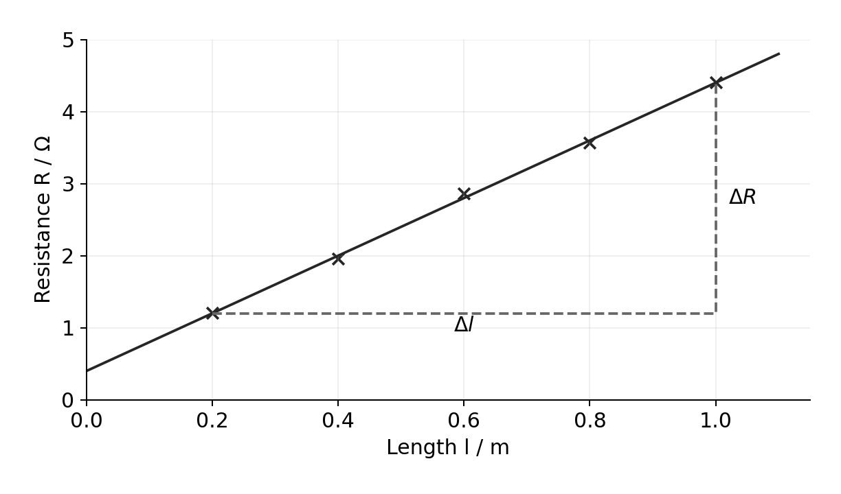
Use distant points on the best-fit line, not a tiny pair of neighbouring data points.
Turn a gradient into a physical constant
For a line $y=mx+c$, identify which part of the physical equation matches $m$ and $c$. A straight line does not prove direct proportionality if its intercept is non-zero.
Worked example. A wire follows $R=(\rho/A)l+R_0$. A best-fit line passes through $(0.20\ \text{m},1.20\ \Omega)$ and $(1.00\ \text{m},4.40\ \Omega)$.
Known: two widely separated points on the fitted line. Why: the slope equals $\rho/A$.
If $A=1.0\times10^{-7}\ \text{m}^2$, the resistivity is:
$$\rho = mA = 4.00\ \Omega\,\text{m}^{-1}\times1.0\times10^{-7}\ \text{m}^2 = 4.0\times10^{-7}\ \Omega\,\text{m}$$
The fixed intercept may represent contact or lead resistance. Dividing one measured $R$ by $l$ would include that offset and give the wrong slope.
Scale factors belong in the gradient
Suppose an axis is labelled $f/\text{MHz}$. A gradient read from that graph has MHz in its units. Convert to Hz before using SI constants. A graph of $f$ against $\sin\theta$ has a dimensionless horizontal axis; its gradient therefore has frequency units. Use degree mode if the measured angle is in degrees.
If a supplied equation is $f=(v/\lambda)\sin\theta$, a graph of $f$ against $\sin\theta$ has gradient $v/\lambda$. Rearrange $v=\lambda\times\text{gradient}$. Do not assume every frequency graph has gradient equal to speed.
Curves, maxima and specific improvements
A broad range first locates a maximum. Then take more closely spaced readings around that region. Repeating one point does not locate the maximum between existing points. Keep the other conditions steady, and consider scatter when quoting the best angle or resistance.
For a motion experiment, a set square can improve a horizontal-distance measurement. For a lamp experiment, a dark enclosure can reduce changing background illumination. For a resonance experiment, approach the loudest sound from both higher and lower frequencies and repeat. Each improvement targets a named limitation.
Conclusions supported by uncertainty
A value with uncertainty describes an interval. Compare that interval with the proposed value, then state what the evidence supports. Agreement within uncertainty does not prove that a material or model is uniquely identified.
Worked example. A measured density is $8.90\ \text{g cm}^{-3}$ with percentage uncertainty $0.9\%$. Could it agree with a proposed value $8.94\ \text{g cm}^{-3}$?
The interval is about $8.82$ to $8.98\ \text{g cm}^{-3}$. The proposed value lies inside it, so the measurement is consistent with that value. It does not prove the object has that composition.
If two model predictions both lie inside the interval, the data does not distinguish them. Reduce the dominant uncertainty or add a different measurement before claiming a unique identification.
Check yourself
Before attempting a written practical problem, check that you can:
turn apparatus names into a usable method with controls and a processing route;
read resolution and correct a known zero offset;
distinguish accuracy, precision, repeatability and reproducibility;
calculate a mean, half range and percentage uncertainty;
plot data, use a large gradient triangle and interpret an intercept;
turn a supplied uncertainty into an interval and give a justified conclusion;
link each improvement to the measurement problem it actually reduces.
Pearson Edexcel IAL Physics WPH14/01, Issue 3 (יולי 2021), הדפסה עמ'28–31 (PDF עמ'32–35).
בניית משפט נאמן לתוכן המקורי לפי דרישות ממוספרות; נורמליזציה של סימון מתמטי מה-PDF המקורי. גבולות דף מקומיים אינם כותרות מפרט רשמיות.
הבן ושתמש ב-impulse FΔt = Δp (חוק השני של ניוטון).
CORE PRACTICAL 9: חקור הכוח הפועל על גוף ושינוי התנע שלו.
יישם שימור תנע ליני במישורים.
CORE PRACTICAL 10: השתמש ב-ICT לניתוח התנגשויות בין כדורים קטנים, כגון כדורי פלדה על שולחן.
קבע האם ההתנגשות היא אלסטית או לא-אלסטית.
גזור ושתמש ב-E_k = p²/(2m) לחלקיק שאינו יחסותי.
מקור: הסיילבוס הבינלאומי של קמבריד'ג'
4.2תנועה מעגלית (הצהרות 87–91)
Pearson Edexcel IAL Physics WPH14/01, Issue 3 (יולי 2021), הדפסה עמ'28–31 (PDF עמ'32–35).
בניית משפט נאמן לתוכן המקורי לפי דרישות ממוספרות; נורמליזציה של סימון מתמטי מה-PDF המקורי. גבולות דף מקומיים אינם כותרות מפרט רשמיות.
בייעץ זווית סטייה ברדיאנים ובמעלות, והמרה ביניהן.
הבן מהירות זוויתית ושתמש ב-v = ωr ו-ω = 2π/T.
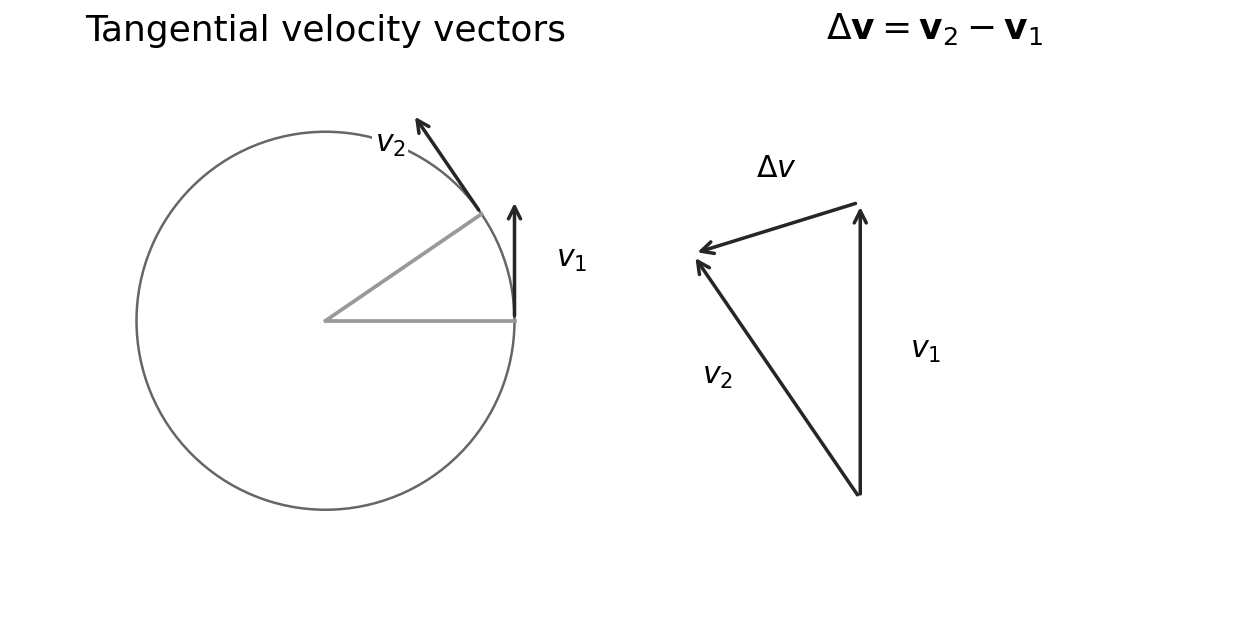
השתמש במדייני וקטורים כדי להסיק את a = v²/r = rω² והשתמש במשוואות אלו.
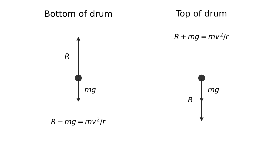
הבן כי כוח צנטריפטלי נטו מייצר ומחזיק בתנועה מעגלית.
השתמש ב-F = ma = mv²/r = mrω².
מקור: הסיילבוס הבינלאומי של קמבריד'ג'
4.3שדות חשמליים ופוטנציאל (הצהרות 92–99)
Pearson Edexcel IAL Physics WPH14/01, Issue 3 (יולי 2021), הדפסה עמ'28–31 (PDF עמ'32–35).
בניית משפט נאמן לתוכן המקורי לפי דרישות ממוספרות; נורמליזציה של סימון מתמטי מה-PDF המקורי. גבולות דף מקומיים אינם כותרות מפרט רשמיות.
הגדר שדה חשמלי כאזור בו חלק טעון חווה כוח.
הגדר והשתמש בעוצמת שדה חשמלי E = F/Q.
השתמש בחוק קולון F = Q₁Q₂/(4πε₀r²).
להשתמש ב-E = Q/(4πε₀r²) למטען נקודתי.
הבן את הקשר בין שדה חשמלי לפוטנציאל.
השתמש ב-E = V/d ללוחות מקבילים.
השתמש ב-V = Q/(4πε₀r) לשדה רדיאלי.
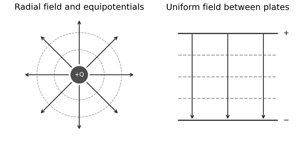
צייר ופרש קווי שדה ואיזופוטנציאלים לשדות אחידים ורדיאליים.
מקור: הסיילבוס הבינלאומי של קמבריד'ג'
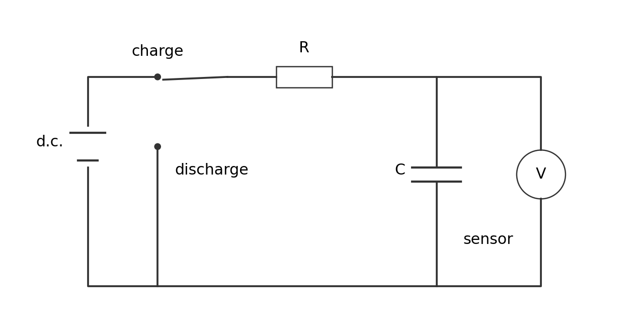
4.4קבלים ומעגלי RC (הצהרות 100–104, CP11)
Pearson Edexcel IAL Physics WPH14/01, Issue 3 (יולי 2021), הדפסה עמ'28–31 (PDF עמ'32–35).
בניית משפט נאמן לתוכן המקורי לפי דרישות ממוספרות; נורמליזציה של סימון מתמטי מה-PDF המקורי. גבולות דף מקומיים אינם כותרות מפרט רשמיות.
הגדר קבלות C = Q/V והשתמש במשוואה זו.
גזור אנרגיה מאוגרת W = ½QV משטח מתחת לגרף פוטנציאל-מטען; גזור והשתמש ב-W = ½CV² וב-W = Q²/(2C).
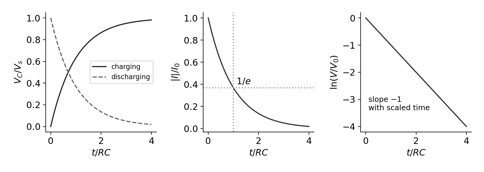
צייר ופרש עקומות טעינה/פריקה של נגד-קבל והבן את קבוע הזמן RC.
מעבדה ליבה 11: השתמש באוסילוסקופ או רשום נתונים להצגת וניתוח המתח על קבל בטעינה ופריקה דרך נגד.
Pearson Edexcel IAL Physics WPH14/01, Issue 3 (יולי 2021), הדפסה עמ'28–31 (PDF עמ'32–35).
בניית משפט נאמן לתוכן המקורי לפי דרישות ממוספרות; נורמליזציה של סימון מתמטי מה-PDF המקורי. גבולות דף מקומיים אינם כותרות מפרט רשמיות.
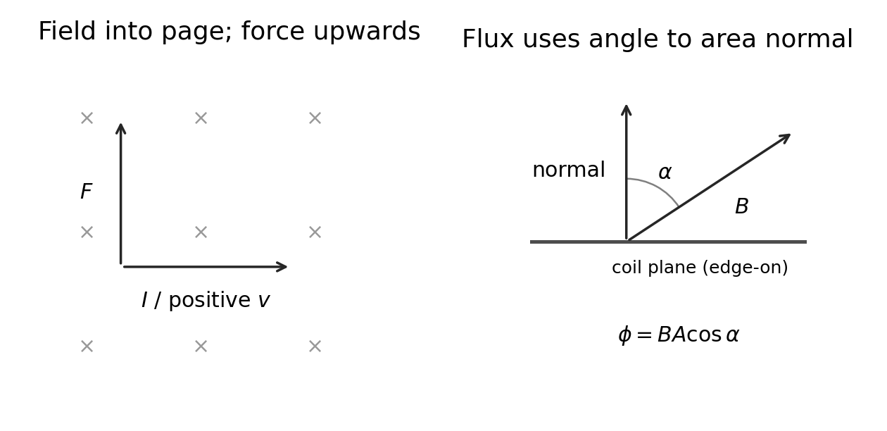
הבן את צפיפות השרות B, הפלוקס φ והקישור הפלוקסי Nφ.
השתמש ב- F = Bqv sinθ והחל את חוק היד השמאלי של פלמי לחלקיקים טעונים.
השתמש ב- F = BIl sinθ והחל את חוק היד השמאלי של פלמי למוליכים.
הבן מה משפיע על כוח חשמלי מופע (e.m.f.) כאשר סליל ומגנט קבוע נעים ביחס זה לזה.
הבן מה משפיע על כוח חשמלי מופע (e.m.f.) כאשר זרם משתנה בסליל אחר הקשור לסליל.
השתמש בחוק פאראדיי ובמשוואה המשולבת של פאראדיי-לנץ: e.m.f. = −d(Nφ)/dt.
Pearson Edexcel IAL Physics WPH14/01, Issue 3 (יולי 2021), הדפסה עמ'28–31 (PDF עמ'32–35).
בניית משפט נאמן לתוכן המקורי לפי דרישות ממוספרות; נורמליזציה של סימון מתמטי מה-PDF המקורי. גבולות דף מקומיים אינם כותרות מפרט רשמיות.
הבן מספר גרעיני (מסה) ומספר אטומי (פרוטונים).
הסבר את עדות פיזור אלפא בזוויות גדולות לדגם הגרעין ואת השינוי ההיסטורי בדגמי האטום.
הבן פליטת תרמית של אלקטרונים והיאצה באמצעות שדות חשמליים ומגנטיים.
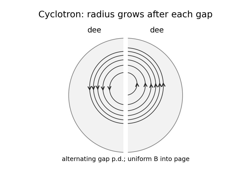
הבן שדות חשמליים/מגנטיים בקוויים, סייקלוטרונים וגלאים; פרטי הגלאים מוגבלים לעקרונות יוניזציה והטיה.
נגזר והשתמש ב- r = p/(BQ) עבור חלקיק טעון בשדה מגנטי.
השתמש בעקרון שימור המטען, האנרגיה והתנע בפעילות חלקיקים ופרשן עקבות.
הסבר מדוע נדרשים אנרגיות גבוהות כדי לחקור את מבנה הגרעון.
הבן עלייה משמעותית יחסית במשך חיי החלקיק; אינה נדרשת שימוש במשוואות יחסיות.
Pearson Edexcel IAL Physics WPH14/01, Issue 3 (יולי 2021), הדפסה עמ'28–31 (PDF עמ'32–35).
בניית משפט נאמן לתוכן המקורי לפי דרישות ממוספרות; נורמליזציה של סימון מתמטי מה-PDF המקורי. גבולות דף מקומיים אינם כותרות מפרט רשמיות.
להשתמש ב-ΔE = c²Δm ביצירת ואיבוד חומר/אנטי-חומר.
להשתמש ב-MeV/GeV לאנרגיה וב-MeV/c² או GeV/c² למסה ולהמיר ליחידות SI.
סווג בריונים (שלושה קווארכים), מזונים (קווארק/אנטי-קווארק), להפטונים בסיסיים ופוטונים; ידוע שהסימטריה במודל חזתה את קווארק העליון.
השתמש בתכונות החלקיק כדי להסיק את תכונות האנטי-חלקיק המתאים ולהפך.
השתמש בעקרון שימור המטען, מספר הבריונים ומספר הלפטונים כדי להעריך פעילויות.
כתוב ופרש משוואות חלקיקים מתוך הסמלים שסופקו.
מקור: הסיילבוס הבינלאומי של קמבריד'ג'
חומר עזר
English
From a collision to a particle accelerator
A car bumper and a particle detector seem very different. Both use momentum and forces. This unit follows those ideas into circular motion, electric fields, magnetic fields and particle interactions.
WPH14 assesses requirements 81–124 of the Issue 3 specification. It can also use knowledge from Units 1–2. Use the seven skill sheets in order. Check units, directions and the assumptions behind each equation. A familiar equation can give a wrong answer when its model does not fit.
Impulse and two-dimensional collisions
Force changes momentum
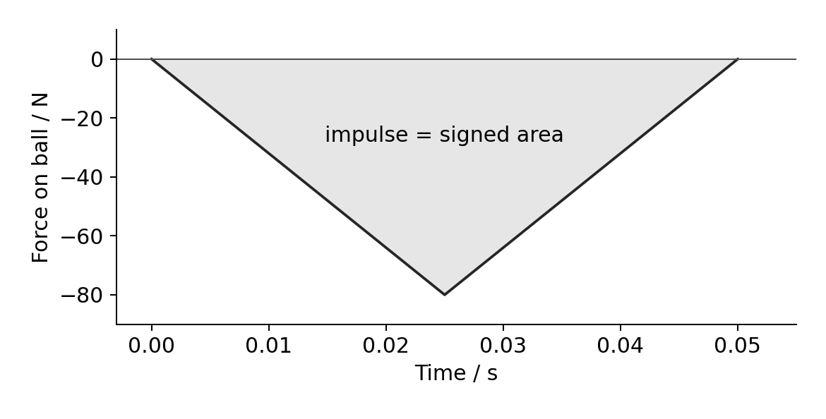
Momentum 动量 is the vector $\mathbf p=m\mathbf v$. Choose a positive direction before using signs. Impulse 冲量 is the change in momentum. For constant force, or the average force over an interval:
$$F_{\text{average}}\Delta t=\Delta p=m(v-u)$$
A changing force gives an impulse equal to the signed area under its force–time graph. A triangular pulse has area $\frac12\times\text{base}\times\text{height}$. An area below the time axis is negative. The maximum force is not automatically the average force.
Worked example. A $0.20\ \text{kg}$ ball approaches a wall at $+6.0\ \text{m s}^{-1}$. It rebounds at $-4.0\ \text{m s}^{-1}$. Contact lasts $0.050\ \text{s}$. Find average force on the ball.
Known: mass, signed initial/final velocities and contact time.
Why: force impulse changes the ball's momentum; rebound reverses the sign.
$$\Delta p=m(v-u)=0.20\ \text{kg}\times(-4.0-6.0)\ \text{m s}^{-1}=-2.0\ \text{kg m s}^{-1}$$
$$F_{\text{average}}=\frac{\Delta p}{\Delta t}=\frac{-2.0\ \text{kg m s}^{-1}}{0.050\ \text{s}}=-40\ \text{N}$$
The force is opposite the chosen positive direction. The wall feels an opposite force. A deforming bumper or helmet increases stopping time. For the same momentum change, this reduces average force. It does not remove the momentum change.
Conserve each momentum component
An isolated system 孤立系统 has no significant external impulse during the event. Its total momentum is conserved. Internal forces cancel in opposite pairs. Momentum conservation does not require kinetic energy conservation.
For a collision in a plane, resolve every momentum into two perpendicular axes:
Use the angle measured from the chosen axis. Include signs; a downward component is negative if upwards is positive. Do not add momentum magnitudes when directions differ.
Worked example. A $0.10\ \text{kg}$ sphere moving at $2.0\ \text{m s}^{-1}$ strikes two stationary spheres, each $0.10\ \text{kg}$. It stops. The two others leave symmetrically at $1.2\ \text{m s}^{-1}$, at angles $+\theta$ and $-\theta$ to the original direction. Find their separation angle and classify the collision.
Why: transverse momenta cancel by symmetry; longitudinal momentum gives $\theta$.
An elastic collision 弹性碰撞 conserves total kinetic energy as well as momentum. An inelastic collision 非弹性碰撞 does not conserve kinetic energy; some becomes other forms of energy.
This collision is inelastic. Total energy is still conserved. In an ordinary passive collision, kinetic energy cannot increase without an additional energy source.
For a non-relativistic particle 非相对论粒子, use $p=mv$ and $E_k=\frac12mv^2$. Substituting $v=p/m$ gives:
At equal kinetic energy, $p=\sqrt{2mE_k}$: a larger mass has larger momentum. At equal momentum, a larger mass has smaller kinetic energy. These equations are not valid for a particle moving close to light speed.
Core practicals 9 and 10
For core practical 9, use a trolley, force sensor and data logger. Measure trolley mass and velocities just before/after contact using light gates or a motion sensor. Record the force–time pulse at a sampling rate fast enough to resolve it. Zero the force sensor; use consistent axes for force and velocity. Integrate the graph area and compare it with $m(v-u)$. Repeat for different contact forces or speeds. A graph of impulse against momentum change should have gradient close to one. Friction, sensor offsets and missed parts of the pulse can cause disagreement. Secure the track and catch the trolley safely.
For core practical 10, record small spheres colliding on a level surface using an overhead camera. Include a length scale in the collision plane and a known frame rate. Keep the camera perpendicular to reduce perspective error. Track centres over several frames before and after the short collision. Convert pixel displacements to metres and frame intervals to seconds. Determine both velocity components, then compare total momentum components and kinetic energies. Repeat with different approach directions. Include uncertainty from positions, timing and scale calibration. A small mismatch within uncertainty is not evidence that momentum fails. Keep spheres contained so they cannot fall or become a slipping hazard.
Circular motion
Angle, angular speed and tangential speed
An angle of one radian 弧度 subtends an arc equal to the radius. Hence $\theta=s/r$, with angle in radians. One revolution is $2\pi$ radians or $360^\circ$.
Angular velocity 角速度 describes the rate of angular displacement. In the plane problems here, use its signed rotational rate or magnitude as appropriate. Points on one rigid turntable have the same angular speed. Points farther from its centre have larger tangential speed 切向速率. Their velocity directions also vary around the circle.
Worked example. A wheel rotates at $120$ revolutions per minute. Find angular speed and acceleration of a point $0.25\ \text{m}$ from its centre.
Keep the unrounded angular speed during the calculation. Use radius, not diameter.
Why acceleration points inward
Uniform circular motion has constant speed but changing velocity. Draw the initial and final tangential velocity vectors. The change is $\Delta\mathbf v=\mathbf v_2-\mathbf v_1$, not their sum. For a small angular change, the velocity triangle and radius triangle are similar:
Centripetal force names the resultant of real forces. It is not an extra force to add to a force diagram. Friction can provide it on a turntable. Tension can provide it for a ball on a string.
Write the real-force equation
For clothing against the inside of a vertical drum, weight always points down. The drum's normal reaction points towards the centre. At constant speed:
The required resultant has the same magnitude, but the reaction is larger at the bottom. If contact is lost, the surface cannot provide a pulling normal reaction. Check this before using a circular-path model.
For a horizontal turntable, the largest available friction must be at least $mr\omega^2$. If maximum friction is $mg/25$:
Mass cancels because both required and available forces scale with mass. If the inward force disappears, motion initially follows the tangent. Gravity can then curve the later path; “tangent” describes the release direction.
Electric fields and potential
Force and potential describe different things
An electric field 电场 is a region where a charged particle experiences a force. Electric field strength 电场强度 is force per unit positive test charge:
Potential is a scalar; field is a vector. A point with zero potential need not have zero field. Adding signed potentials is different from adding field vectors.
Radial and uniform fields
For point charges, or outside an isolated charged conducting sphere, with $k=1/(4\pi\varepsilon_0)$:
Here $r$ is separation of charge centres; sphere distances are measured from its centre. Like charges repel, unlike charges attract. Potential takes the sign of $Q$ when zero is at infinity.
Between large parallel plates, away from edges, the field is approximately uniform:
$$|E|=\frac{|\Delta V|}{d}$$
The field points from higher to lower potential. Plate separation $d$ is perpendicular to the plates. An equipotential 等势面 has the same potential everywhere. Field lines cross equipotentials at right angles. Moving along one involves no change in electric potential energy.
The radial field is the negative potential gradient: $E_r=-\mathrm dV/\mathrm dr$. For a positive source, the signed area under its $E$–$r$ curve from $r$ to infinity equals $V(r)$. The area from zero to $r$ is not that potential. In a uniform field, closer equally spaced potential levels mean stronger field.
Worked example. A sphere of radius $0.20\ \text{m}$ has potential $9.0\ \text{kV}$. Find charge and field at $0.30\ \text{m}$ from its centre. Use $k=8.99\times10^9\ \text{N m}^2\text{C}^{-2}$.
Use the surface radius to find charge, then the new centre-distance to find field. Do not reuse the surface distance for the second step.
Compare electrical and gravitational forces
A stationary charged oil drop can satisfy $|q|E=mg$. Use $m=\rho\mathcal V$ if density and volume are given. Divide the charge magnitude by $e=1.60\times10^{-19}\ \text{C}$ to test whether it is close to an integer multiple. Charge sign follows the direction of force required, not its magnitude alone.
To lift a spherical grain, compare $qE$ with $\rho(4\pi r^3/3)g$. Radius is half the listed diameter. A calculated maximum diameter is a threshold: choose the largest listed diameter below it. On an inclined panel, the normal component of weight is $mg\cos\theta$. The electric force perpendicular to the panel need overcome that component to detach a grain; gravity also has a downslope component.
Capacitors and RC circuits
Charge storage and energy
A capacitor 电容器 stores separated charge on two conductors. They carry equal and opposite charges in the ideal two-plate model. The quoted charge $Q$ is the magnitude on either plate, not the sum of both magnitudes. Capacitance 电容 is charge stored per unit p.d.:
$$C=\frac QV$$
One farad is one coulomb per volt. For constant capacitance, a $V$–$Q$ graph is straight through the origin with gradient $1/C$. Its area gives the work needed to transfer charge onto the capacitor:
$$W=\frac12QV=\frac12CV^2=\frac{Q^2}{2C}$$
The factor one half appears because p.d. rises from zero while charge is transferred. It is not $QV$ at the final voltage throughout charging. For discharge between non-zero voltages, subtract the two stored energies:
This is different from $\frac12C(V_{\text{initial}}-V_{\text{final}})^2$.
Charging and discharging
In an ideal series resistor–capacitor charging circuit, initially uncharged, the capacitor p.d. is zero. The resistor initially has the full supply p.d., so current is maximum. As charge builds, capacitor p.d. rises. Resistor p.d. and current fall. At full charge, current is zero and capacitor p.d. equals supply p.d.
For discharge through a fixed resistance, use signed current consistently or work with its magnitude:
The voltage relation follows from $Q=CV$ with constant $C$. Current magnitude follows from $|I|=V/R$ with constant $R$. The time constant 时间常数 is $\tau=RC$. After one time constant, $Q$, $V$ and current magnitude are $e^{-1}\approx0.368$ of their initial values. After three time constants they are about $5\%$, not zero. Stored energy falls faster because it depends on $V^2$.
A charging capacitor voltage rises towards $V_s$; charging current falls towards zero. Do not sketch the same curve for both quantities. Equal $V_C$ and $V_R$ means each is $V_s/2$, reached at $t=RC\ln2$.
Taking natural logs of the discharge equation gives:
$$\ln V=\ln V_0-\frac{t}{RC}$$
Thus a graph of $\ln V$ against $t$ has gradient $-1/(RC)$ and intercept $\ln V_0$. The same forms hold for $Q$ and current magnitude. Use consistent measurement units inside the logged numerical values.
Worked example. A $100\ \mu\text{F}$ capacitor discharges from $12.0\ \text{V}$ through $20.0\ \text{k}\Omega$. Find p.d. after $3.0\ \text{s}$ and energy lost.
The lost stored energy becomes mainly heat in the discharge resistance. Use unrounded voltage in the final calculation.
Core practical 11 and useful extensions
Use a low-voltage d.c. supply, resistor, capacitor and switch. Charge through the resistor, then disconnect the supply and discharge through the known resistance. Connect a voltage sensor, data logger or oscilloscope across the capacitor. Record time and p.d.; choose a sampling interval short compared with $RC$. Use an instrument input resistance large compared with the discharge resistance, otherwise it changes the discharge path.
Keep $R$ and $C$ fixed, repeat after restoring the same initial charge, and compare measured curves with exponential predictions. Determine $RC$ from the $1/e$ level or a log-fit gradient. Avoid taking logs of readings near zero where relative uncertainty is large. For a resistance-tolerance test, calculate $R=-\Delta t/[C\ln(V_2/V_1)]$ during one uninterrupted discharge and compare with both limits of the permitted interval.
Use correct polarity for an electrolytic capacitor and remain below its voltage rating. Discharge it safely through a resistor before altering connections; do not short a charged capacitor. Leakage, sensor loading and resistor heating can change the measured curve.
A smoothing capacitor charges near supply peaks and discharges into the load between them. A smaller load resistance gives a smaller time constant, faster discharge and less smoothing. For two identical series capacitors, the same magnitude of charge appears on each. Their equal p.d.s share the supply, so each stores half the charge of one identical capacitor connected alone. This sharing is a useful bridge to the selected paper; it does not replace the main capacitance model.
Magnetic forces and induction
Directions, flux and force
Magnetic flux density 磁感应强度$B$ describes the field's force effect. For a straight wire of length $l$ in a uniform field:
$$F=BIl\sin\theta$$
Here $\theta$ is between conventional current and field. Only the length inside the field counts. For one charged particle:
$$F=|q|vB\sin\theta$$
Use Fleming's left-hand rule 弗莱明左手定则: first finger along field, second along conventional current, thumb gives force. A positive charge moves with conventional current. Reverse the result for an electron's motion. Dot symbols mean out of the page; crosses mean into it.
Magnetic force is perpendicular to velocity, so it changes direction without doing work. It cannot, alone, increase the particle's kinetic energy. If $\mathbf v$ is parallel to $\mathbf B$, magnetic force is zero.
Magnetic flux 磁通量 through a flat area in a uniform field is:
$$\phi=BA\cos\alpha$$
Here $\alpha$ is between field and the area's normal, not the plane itself. The unit is the weber. Flux linkage 磁通链 is $N\phi$ when the same flux links each of $N$ turns.
Worked example. A coil has 40 turns and radius $0.015\ \text{m}$. A uniform $0.020\ \text{T}$ field is perpendicular to its plane. Find flux linkage.
Use radius, not diameter, and multiply by turns only when finding linkage. A balance under magnets measures the opposite reaction to a force on a separately supported wire. Convert a balance reading change $\Delta m$ to force $\Delta mg$, not $\Delta m$ itself.
A changing linkage induces an e.m.f.
Electromagnetic induction 电磁感应 occurs when flux linkage changes. Relative movement of a coil and magnet can cause it. Rotating the coil or changing current in another linked coil can also cause it. A stationary coil in a constant field has no induced e.m.f. merely because flux is present.
Faraday's law 法拉第电磁感应定律 relates e.m.f. magnitude to rate of flux-linkage change. Lenz's law 楞次定律 gives the opposing direction:
Induced current, if the circuit is closed, produces a magnetic effect opposing the change that caused it. It does not always oppose the existing field: when that field decreases, the induced effect helps maintain it. This opposition is consistent with energy conservation.
Worked example. Flux through each of 50 turns decreases from $6.0\times10^{-5}$ to $2.0\times10^{-5}\ \text{Wb}$ in $0.020\ \text{s}$. Find average induced e.m.f. magnitude.
Faster movement, stronger field, more turns or larger linked area can increase the rate. Explain which quantity actually changes. In a magnetic-strip reader, reversing pole orientation reverses signal direction. For a straight boundary swept across an area of width $L$ at speed $v$, $\Delta A/\Delta t=Lv$, giving $|\mathcal E|=NBLv$ under that uniform-field model.
Wireless charging uses alternating current in one coil, producing changing magnetic field and changing linkage in the phone coil. That induces an e.m.f. The receiving circuit can then charge the battery. Equal turn counts do not ensure equal voltages: some flux may fail to link the other coil, especially with separation or without an iron core.
Nuclear structure, accelerators and tracks
The nucleus and scattering evidence
In $^{A}_{Z}X$, proton number 质子数$Z$ counts protons and nucleon number 核子数$A$ counts protons plus neutrons. The neutron count is $A-Z$. A neutral atom has $Z$ electrons; an ion need not.
The older distributed-positive-charge model could explain small deflections but not the observed rare large-angle alpha scattering. Most alpha particles pass nearly straight through thin foil, showing that most of the atom is empty space. A small fraction experience very large deflections. Positive alpha particles feel strong electrostatic repulsion near a small, dense, positive nucleus containing most atomic mass. Few large-angle events show that the nucleus occupies a small fraction of the atom's volume. Keep each observation linked to the particular conclusion it supports.
Make, accelerate and steer a beam
Thermionic emission 热电子发射 releases electrons from a heated metal. Heating supplies energy so some electrons can leave the surface. A positive accelerating electrode attracts them through a vacuum. A potential difference changes kinetic energy by the electric work:
For speed calculations use the positive energy gain $|q|\,|\Delta V|$ only when the particle is accelerated through the field in the appropriate direction. Starting from rest, well below light speed:
$$\frac12mv^2=|q|\,|\Delta V|$$
A linear accelerator 直线加速器 uses alternating p.d. across gaps between drift tubes. Particles accelerate in gaps and are shielded inside the conducting tubes. The polarity reverses while particles are inside, so the next gap accelerates them again. At constant alternating frequency, increasing speed requires longer tubes to maintain the time between successive gaps. Across $n$ equal accelerating gaps, total kinetic-energy gain is $n|q|V_{\text{gap}}$.
A cyclotron 回旋加速器 uses a magnetic field perpendicular to two hollow dees. Electric field accelerates particles across the gap. Inside a dee, magnetic force curves the path without increasing speed. Polarity reverses during each half-turn, allowing another energy gain at the next crossing. With perpendicular entry:
In the non-relativistic model, the period is independent of speed. Increasing speed increases radius. Time in one dee is $T/2$, not $T$. The formula assumes constant field and fixed mass in this model; synchronisation fails as relativistic effects become important.
Worked example. A proton moves perpendicular to $B=0.40\ \text{T}$ with momentum $2.0\times10^{-20}\ \text{kg m s}^{-1}$. Use proton mass $1.67\times10^{-27}\ \text{kg}$.
When starting instead from a de Broglie wavelength, use $p=h/\lambda$, then $E_k=p^2/(2m)$ and $V=E_k/|q|$. Check that the non-relativistic assumption remains suitable.
Read detector evidence carefully
Charged particles ionise matter along their paths, leaving detectable tracks. A neutral particle does not make a direct ionisation track in this model. Its presence can be inferred from missing momentum or from charged products it later produces.
In a known perpendicular magnetic field, curvature direction together with travel direction can identify charge sign. Without field direction, curvature alone cannot give sign. Radius gives momentum through $p=B|q|r$; comparing radii requires knowledge of charge magnitude. A tightening track often shows momentum being lost. Do not infer travel direction from a constant-radius arc alone.
Conserve charge, total energy and vector momentum at an interaction. If visible outgoing momenta do not add to the incoming momentum, a neutral product may carry the missing component. Draw a vector balance rather than guessing from the number of tracks.
High energies probe nucleon structure in two ways. Large momentum gives a short de Broglie wavelength, allowing small structure to be resolved. High collision energy also allows new massive particles to be created. Quarks are not observed as isolated free particles; do not describe a high-energy collision simply as removing a free quark.
Fast muons can reach the ground because their average lifetime measured in the Earth's frame is increased at speeds close to $c$. This does not mean they exceed light speed. Unit 4 requires the significance of this lifetime increase, not use of relativistic equations.
Particles, antiparticles and conservation
Families and antiparticles
In the quark–lepton model 夸克—轻子模型, baryons and mesons contain quarks. Leptons are fundamental particles in the model.
A baryon 重子 contains three quarks, for example a proton $uud$ or neutron $udd$. An antibaryon contains three antiquarks.
A meson 介子 contains one quark and one antiquark, for example a pion.
A lepton 轻子 is fundamental, for example an electron or neutrino. A positron is an antilepton, not a meson.
A photon is the quantum of electromagnetic radiation; it is neither a baryon nor a lepton.
Up-type quarks have charge $+2e/3$ and down-type quarks $-e/3$. Antiquarks have opposite charges. For example, $uud$ sums to $+e$ and $udd$ to zero. The symmetry of the quark families predicted a top quark before it was observed. Classification models make testable predictions, not just lists of known particles.
An antiparticle 反粒子 has the same rest mass as its particle and opposite electric charge when charged. Other relevant additive quantum numbers also reverse. An electron has lepton number $+1$; its positron has $-1$. Both have baryon number zero. A neutral antiparticle can differ in quantum numbers despite having no electric charge.
Check conserved totals
Assign baryon number $+1$ to a baryon, $-1$ to an antibaryon, and zero to mesons/leptons/photons. Quarks carry $+1/3$ and antiquarks $-1/3$. Assign lepton number $+1$ to a lepton and $-1$ to an antilepton. Compare total charge, baryon number and lepton number on both sides of a proposed reaction. Also check energy and momentum. Passing the listed conservation checks alone does not prove that an interaction will occur; it establishes that those laws do not forbid it.
Worked example. Test $n\rightarrow p+e^-+\bar\nu_e$.
Quantity
Before
After
Charge / $e$
0
$+1-1+0=0$
Baryon number
1
$1+0+0=1$
Lepton number
0
$0+1-1=0$
The antineutrino balances the electron's lepton number. Changing it to a neutrino would make the final total $+2$, so that proposed equation would fail this check. Preserve bars and charge signs when interpreting supplied particle symbols.
Rest energy, creation and annihilation
Mass–energy equivalence 质能等价 relates a rest-mass change to energy:
$$\Delta E=c^2\Delta m$$
In pair production 粒子对产生, energy creates a particle–antiparticle pair. The energy must at least supply both rest masses; extra energy can become kinetic energy or recoil. Momentum must also be conserved, so the surrounding interaction matters. In annihilation 湮灭, particle and antiparticle can turn into photons. A pair initially at rest producing two photons gives equal photon energies and opposite momenta. Each photon carries one particle's rest energy for an equal-mass pair; the total is twice that value.
One electronvolt is $e$ joules: $1\ \text{eV}=1.60\times10^{-19}\ \text{J}$. MeV means $10^6$ eV and GeV means $10^9$ eV. A quoted mass in $\text{MeV}/c^2$ is a mass unit, not an energy unit. Multiply by $c^2$ to get its corresponding rest energy.
Worked example. Convert a mass of $140\ \text{MeV}/c^2$ to kilograms.
Use the same units before comparing masses. Percentage difference from an accepted value is $100\times|m_{\text{predicted}}-m_{\text{accepted}}|/m_{\text{accepted}}$. State the reference value. In threshold questions, distinguish rest-energy supply from kinetic energy; do not use $p=mv$ for a photon or a particle close to $c$.
Check yourself
Can you use signed impulse and two momentum components, then test kinetic energy separately?
Can you derive centripetal acceleration and draw only actual forces?
Can you distinguish field vectors, signed potential and energy changes?
Can you choose the correct capacitor curve and use log slope or tolerance evidence?
Can you explain induction as a change in linkage, including the opposing direction?
Can you separate electric acceleration from magnetic steering and halve a cyclotron period correctly?
Can you preserve particle symbols, conservation totals and energy/mass units?
The skill sheets develop these methods before authentic past-paper tasks. Original practice also covers requirements not sampled in the two recent papers. A short sample of authentic questions does not define the whole syllabus.
קיבולת חום ספציפית/חום נסתר; אנרגיה פנימית; הבדל בין העברת אנרגיה לטמפרטורה. CP12 כיול תרמיסטור/מחלקת מתח ו-CP13 חום נסתר עם קלט חשמלי, אובדן מסה ותיקון אובדן.
הוכחה דורשת אחורית: plans/2026-10-09-edexcel-ial-physics-u5-demand-map.md. מבחן יחידה 5 הוא סינתטי עם היחידות 1, 2 ו-4.
אפס מוחלט וקלวิน; pV=NkT, יחסים בכמות קבועה; CP14 לחץ/נפח בטמפרטורה קבועה; נגזור אנרגיה קינטית תנועתית ממוצעת מולקולרית 3kT/2 מהתיאוריה הקינטית, והבדל בין מהירות RMS ומהירות ריבועית ממוצעת.
הוכחה דורשת אחורית: plans/2026-10-09-edexcel-ial-physics-u5-demand-map.md. מבחן יחידה 5 הוא סינתטי עם היחידות 1, 2 ו-4.
כוח מחזיר פרופורציונלי הפוך להזזה; קשרי x,v,a סימניים ופאזה, תקופות קפיץ/מתלה, שיפועי גרף, החלפת אנרגיה ללא ריכוך ואובדן אנרגיה מרוכך. CP16 זיהוי מסה לא ידועה מתדרוני תהודה עם מסות ידועות מכולות.
הוכחה דורשת אחורית: plans/2026-10-09-edexcel-ial-physics-u5-demand-map.md. מבחן יחידה 5 הוא סינתטי עם היחידות 1, 2 ו-4.
עקומות גוף שחור, חוקי סטפן-בולצמן וויין, בהירות/עוצמה, רדיוס מול שטח, פרלוקס טריגונומטרי ורזולוציה, נרות סטנדרטיים, צירים/אזורים ב-HR ואופן מחזור חיי הכוכבים.
הוכחה דורשת אחורית: plans/2026-10-09-edexcel-ial-physics-u5-demand-map.md. מבחן יחידה 5 הוא סינתטי עם היחידות 1, 2 ו-4.
מנגנון דופלר, קונבנציות אורך גל/תדר להזזה אדומה, v/c לא-יחסותי מקובל, חוק האבל ויחידות, הנחות זמן 1/H0, מחלוקת גיל/גורל וחומר אפל; הימנעו מהתייחס למסמך מדוגם כטווח מלא.
הוכחה דורשת אחורית: plans/2026-10-09-edexcel-ial-physics-u5-demand-map.md. מבחן יחידה 5 הוא סינתטי עם היחידות 1, 2 ו-4.
מקור: הסיילבוס הבינלאומי של קמבריד'ג'
חומר עזר
מקרר גלידה לכוכב
קרר גלידה, גשר מתנדנד וכוכב רחוק כולם מעורבים באנרגיה. יחידה זו מקשרת בין תנועת מולקולרית, שינויים גרעיניים, תנודות ותצפיות אסטרונומיות. המשימה היא לעיתים לבדוק טענה, ולא רק לחשב מספר: לנסח את הדגם, להעביר יחידות לאורך החישוב, ולשוות את התוצאה עם הטענה.
WPH15 מכסה הצהרות 125–171 מבעיית Pearson 3. הוא משתמש גם ביחידות 1, 2 ו4. עברו על דפי 5.1–5.9 לפני סטות האמיתיות המתאימות להן. השתמשו בקבועים הסופקו באופן עקבי: $g=9.81\ \mathrm{m\,s^{-2}}$, $k_B=1.38\times10^{-23}\ \mathrm{J\,K^{-1}}$ ו$G=6.67\times10^{-11}\ \mathrm{N\,m^2\,kg^{-2}}$ אלא אם כן השאלה נותנת ערך מקומי שונה. כאן $k_B$ הוא קבוע בולצמן; $k_s$ מציינת קבוע קפיץ.
חימום, שינוי פאזה וכיול תרמיסטור
עקבו אחרי האנרגיה, לא רק אחרי הטמפרטורה
אנרגיה פנימית היא סך האנרגיה בתנועה האקראית ובאינטראקציות המולקולריות: אנרגיה קינטית אקראית פלו אנרגיה פוטנציאלית בין-מולקולרית. היא אינה כוללת את האנרגיה הקינטית של כל הגוף הנע יחד. טמפרטורה קשורה לאנרגיה הקינטית האקראית הממוצעת של המולקולות, ולא לאנרגיה הפנימית הכוללת. שתי דגימות בטמפרטורה זהה יכולות להיות בעלות אנרגיות פנימיות שונות משום הכמות והמצב שלהם שונים.
קיבולת חום סגולית$c$ היא האנרגיה הנדרשת לכל ק"ג למעלה של קלווין אחת ללא שינוי מצב. חום סתום סגולי$L$ הוא האנרגיה המועברת לכל ק"ג במהלך שינוי מצב ספציפי בטמפרטורה קבועה.
הבדל טמפרטורות של $1\ ^\circ\mathrm C$ שווה להבדל של $1\ \mathrm K$. טמפרטורות מוחלטות בחוקי גזים וקרינה חייבות להיות בקלווין. במהלך התמסה או רתיחה, אנרגיה משנה את סידורי המולקולות ואנרגיה פוטנציאלית בעוד שהטמפרטורה נשארת קבועה בשינוי פאזה אידיאלי בטמפרטורה קבועה. קרר גלידה סופח אנרגיה מהאוכל/סביבה כאשר הוא נמס. הוא אינו שולח "אנרגיה קרה" לתוך האוכל.
עם הספק חימום קבוע, שיפולים תלולים יותר בטמפרטורה-זמן מצביעים על קיבולת חום סגולית קטנה יותר $mc$, בהנחה שאובדן חום זניח. חלק שטוח אינו אומר שהעברת אנרגיה הפסיקה. עבור מחמם, האנרגיה הנכנסת היא $E_{\rm in}=Pt=VIt$; אנרגיה תרמית מועילה יכולה להיות קטנה יותר משום שאנרגיה בורחת לסביבה.
דוגמה מופיעה. קוביית קרח בגובה $0.40\ \mathrm{kg}$ בטמפרטורת $-10\ ^\circ\mathrm C$ נמסה למים בטמפרטורת $0\ ^\circ\mathrm C$. השתמשו ב$c_{\rm ice}=2100\ \mathrm{J\,kg^{-1}\,K^{-1}}$ וב$L_f=3.4\times10^5\ \mathrm{J\,kg^{-1}}$.
נתון: מסה, טמפרטורות התחלתיות/סופיות וקבועי חומר. מדוע: חימום המוצק והתמסתו הם העברות אנרגיה נפרדות.
דוגמה מופיעה. מחמם בגובה $1000\ \mathrm W$ מרתיח $0.20\ \mathrm{kg}$ מים בזמן של $600\ \mathrm s$. מצאו יעילות, באמצעות ⟨$L_v=2.26\times10^6\ \mathrm{J\,kg^{-1}}$⟩.
עבור טעינות קומקום חוזרות, חשבו נפח מים כולל, מספר טעינות וזמן פעולה כולל. השווו אנרגיות לאורך אותו מרווח זמן מצויין. אובדן במצב המתנה לאורך יום והכניסה הנדרשת להרתיח מים הם כמויות שונות; ציינו מה שהשוואה מסוימת מקימה למעשה.
CP12: כיול תרמוסטט
לתרמיסטור יש התנגדות משתנה עם הטמפרטורה. תרמיסטור הנפוץ בעל מקדם טמפרטורה שלילי (NTC) מקטן בהתנגדות כאשר מתחמם. במחלקת מתח:
כאשר התרמיסטור הוא ההתנגדות התחתונה והמתח נמדד על פיו, החימום מקטין את מתח הפלט. החלפת מיקום ההתנגדות הופכת מגמה זו. תרמוסטט מתפעל ברף מתח פלט נבחר; מחלקת מתח לבדה אינה מכשיר הפעלה מלאך.
למעשה ליבה 12, מניחים את התרמיסטור ואת מדחום התייחסות סמוך זה לזה באמבט מים מעורבב. שומרים על מגעים חשמליים יבשים ומבודדים. בטמפרטורות שונות בתוך הטווח הרצוי, מחכים לאיזון תרמי ומדויקים טמפרטורה ומתח מחלק. שמרים על מתח האספקה וההתנגדות הקבועה ללא שינוי. משתמשים במולטימטר בעל התנגדות כניסה גבוהה כדי להפחית עומס. מציירים את המתח נגד הטמפרטורה ומעריכים את המתח עבור טמפרטורת ההפעלה הנבחרת. חוזרים על הקריאות או משווים חימום/קירור לגילוי השהיה. אין להניח קליברציה ליניארית ללא ראיות. משתמשים בחשמל בעל מתח נמוך ונוטים זהירות עם מים חמים.
CP13: מדידת חום טמיעה
אספקת הספק חשמלי נמדד לחומר במהלך מעבר פאזה. מדידת מסת המסה או האידוי במרווח זמן נתון לאחר ייצוב התנאים. מאזן מודד שינוי במסה; אין לבלבל בין נפח הנוזל שנאסף לבין המסה. ללא תיקון אובדנים, $L=VIt/\Delta m$ מניח כי כל האנרגיה שהוספקה גורמת למעבר הפאזה.
תיקון שימושי הוא השוואה בין שני הספקים בטמפרטורת מעבר פאזה יציבה אותה. אם הספק אובדן החום הוא בקירוב ללא שינוי, חיסור בין שתי המדידות מבטל אותו:
$$L=\frac{P_2-P_1}{\dot m_2-\dot m_1}$$
לשנות את הנחת אובדן קבוע. מדידת ביקורת של התכה ללא הגוף המחמם היא תיקון אפשרי נוסף בניסוי קרח מתאים. מפחיתים אובדן חום באמצעות בידוד במקום בטוח; נמנעים מהתזה, משטחים חמים ומחברות רשת לא בטוחות.
גזים אידיאליים ואנרגיה קינטית מולקולרית
קלווין ומודל הגז האידיאלי
אפס מוחלט הוא $0\ \mathrm K$, כ-$-273\ ^\circ\mathrm C$. זוהי הגבול התחתון של הטמפרטורה התרמודינמית. במודל הגז האידיאלי הקלאסי, אנרגיה קינטית תרגולית ממוצעת שואפת לאפס כאשר הטמפרטורה שואפת לאפס. גזים אמיתיים צופים לפני שהאקסטרפולציה הזו מושגת; אין לטעון שמולקולות בכל חומר אמיתי מאבדות את כל האנרגיה האפשרית שלהן.
טמפרטורה מוחלטת נמדדת בקלווין: $T=\theta_{^\circ\mathrm C}+273$ בדיוק הנפוץ כאן. גז אידיאלי מורכב ממולקולות בעלות נפח זניח, ללא כוחות ביני-מולקולריים פרט במהלך התנגשויות אלסטיות, ותנועה אקראית. הלחץ נובע משינויי תנע בקירות.
$$pV=Nk_BT$$
כאן $N$ הוא מספר המולקולות, ולא מספר המולים. משתמשים בלחץ בפסקלים, נפח במטר מעוקב וטמפרטורה בקלווין. עבור מספר קבוע של מולקולות:
$$\frac{p_1V_1}{T_1}=\frac{p_2V_2}{T_2}$$
בנפח קבוע, הלחץ פרופורציונלי לטמפרטורה בקלווין. בטמפרטורה קבועה, $pV$ הוא קבוע. יש לכלול את הלחץ החיצוני אם מדחום דוחה על לחץ ביחס לאטמוספירה.
דוגמה מפורטת. מיכל קשיח $2.0\times10^{-3}\ \mathrm{m^3}$ מכיל גז בטמפרטורה $1.0\times10^5\ \mathrm{Pa}$ ולחץ $300\ \mathrm K$. מצאים $N$ ולחץ לאחר חימום ל$360\ \mathrm K$.
אם למולקולה אחת יש מסה $m_0$, מסת הגז הכוללת היא $Nm_0$. עבור כדור, מוצאים תחילה $V=4\pi r^3/3$; הרדיוס הוא חצי הקוטר.
נגזרת הקשר האנרגטי המולקולרי
הקשר לחץ מתורת הקינטיקה הוא $pV=\tfrac13Nm_0\langle c^2\rangle$, כאשר $\langle c^2\rangle$ היא מהירות ריבועית ממוצעת. נובעת משינויי תנע אלסטיים בקיר ובמהירות ממוצעת ריבועית שווה בשלושה כיוונים מאונכים. מהירות ארבעית ממוצעת היא $c_{\rm rms}=\sqrt{\langle c^2\rangle}$; היא אינה ריבוע המהירות הממוצעת.
לקובייה בעלת צלע $l$, מולקולה אחת עם רכיב מהירות $c_x$ משנה תנע קיר ב-$2m_0c_x$ בכל התנגשות אלסטית. זמן החזרה שלה לקיר אותו הוא $2l/c_x$. מכאן הכוח הממוצע שלה הוא $m_0c_x^2/l$. סכום על פני כל המולקולות וחלוקה בשטח הקיר $l^2$:
תנועה אקראית מחולקת באופן שווה בין הכיוונים המאונכים, ולכן $\langle c^2\rangle=3\langle c_x^2\rangle$. זה נותן את קשר הלחץ לעיל. השוו את שני הביטויים ל$pV$, בצעו ביטול של $N$, ולאחר מכן סדרו מחדש:
בטמפרטורה נתונה, מיני גזים שונים יש להם אנרגיות קינטיות תרגוליות ממוצעות שוות, אך מולקולות קלות יותר יש להן מהירויות RMS גדולות יותר. אם המהירות משתנה פי שניים באותה טמפרטורה, מסת המולקולה היא רבע. חימום מגדיל את האנרגיה הקינטית המולקולרית הממוצעת; הוא אינו נותן לכל מולקולה את אותה מהירות.
CP14: לחץ ונפח בטמפרטורה קבועה
כלאו כמות קבועה של גז במצית או בצינור מדוד המחובר לחיישן לחץ. בדוק את כיול הציוד והשתמש בלחץ מוחלט. כלול נפח מתה בצינור החיבור כאשר הוא משמעותי. שנה את הנפח בהדרגה, המתן לאחר כל שינוי עד הטמפרטורה תחזור לסביבה, ולאחר מכן רשום זוגות לחץ–נפח מרובים. אל תשחרר גז. גרף של $p$ נגד $1/V$ אמור להיות ישר העובר בראשית התאמים לתחומי השגיאה. עקומה של $p$–$V$ אינה ישרה. הימנע מלחץ גבוה מדי וחבר את החיבורים היטב. הדחקה מהירה מחממת את הגז ומפרה את תנאי הטמפרטורה הקבועה הרצוי.
אנרגיית קישור, התפוררות והיתוך
חוסר מסה הוא הפרש אנרגיה
ליבת אטום מכילה $Z$ פרוטונים ו$A-Z$ נייטרונים. המסה שלה קטנה ממס הכוללת של ניוקליונים חופשיים אלו. חוסר המסה זה מתאים ל-אנרגיית הקישור הנדרשת כדי להפריד את הליבה לחלוטין לניוקליונים חופשיים:
$$\Delta m=Zm_p+(A-Z)m_n-m_{\rm nucleus}\qquad E_b=\Delta m c_0^2$$
כאן $c_0$ היא מהירות האור, הנבדלת מקיבול החום הספציפי. יחידת המסה האטומית המאוחדת היא $1\ \mathrm u=1.66\times10^{-27}\ \mathrm{kg}$. המר כל המסות ליחידה אחידה לפני ביצוע החיסור. מסות גרעיניות ומסות אטומים ניטרליים אינן חלופיות זו בזו ללא התחשבות עקבית באלקטרונים. השתמש במסות שמדויק מסופקות בשאלה.
$$1\ \mathrm{MeV}=1.60\times10^{-13}\ \mathrm J\qquad \text{binding energy per nucleon}=E_b/A$$
דוגמה פותרת. ליבה יש חוסר מסה $0.030\ \mathrm u$ ו$A=4$. מצא את אנרגיית הקישור לכל ניוקליון.
עקומת אנרגיית הקישור לכל ניוקליון עולה בחוד למימניות קלות, מגיעה לשיא בסביבות ברזל/ניקל, ולאחר מכן יורדת בהדרגה למימניות כבדות. אנרגיית קישור גדולה יותר לכל ניוקליון משמעת בדרך כלל שהניוקליונים קשורים חזק יותר. הערך האנכי, ולא רק מסה אטומית, הוא מה שחשוב בעת השוואת נקודות.
היתוך גרעיני מאחד מימניות קלות. התפוררות גרעינית מפצל ליבה כבודה לתוצרים קטנים יותר, לעיתים עם נייטרונים. אנרגיה משתחררת כאשר לתוצרים יש אנרגיית קישור כוללת גדולה יותר ומסת ריפוד כוללת קטנה מזו של המגיבים. עבור תגובה, חשב את הפרש המסה הכולל, ולא רק הפרש בין שתי ערכים של אנרגיית קישור לכל ניוקליון. אנרגיה כוללת שמורה.
היתוך דורש טמפרטורה גבוהה מאוד כדי לספק לניוקליונים מספיק אנרגיה קינטית להתקרב למרות הדחייה האלקטרוסטטית, וצפיפות/כליא גבוהה כדי לבצע מספיק פגישות קרובות ולשמור על שחרור אנרגיה. לטמפרטורה ולצפיפות יש תפקודים שונים. פשוט לציין "לחץ גבוה" אינו מסביר את הפיכת ההדחה.
קרינה, רקע ודעיכה
בחר קרינה לפי האינטראקציה שלה
קרינת אלפא מורכבת מליבות הליום: יוננות חזקה, טווח קצר ועוצרה על ידי נייר או כמה סנטימטרים של אוויר. קרינת בטא מורכבת מאלקטרונים או פוזיטרונים: פחות יוננת, חדירה יותר, בדרך כלל עצורה על ידי כמה מילימטרים של אלומיניום. קרינת גמא היא קרינה אלקטרומגנטית: יוננות חלשה וחדירה מאוד; עופרת או בטון מפחיתים את עוצמתה אך לא מספקים עובי עצירה חד.
בתא ערפל, מעברים של אלפא הם עבים בעיקר בגלל היונות החזקה, ויחסית ישרים כי לחלקיקים יש מסה גדולה בהשוואה לחלקיקי בטא. מעברי בטא הם צרים ונדחים בקלות יותר. אל תחליף הסברים אלו. קרינת בטא יכולה לשמש לניטור עובי נייר מכיוון שחלק מהחלקיקים עוברים וחלקם נבלעים; שינוי בעובי משנה את קצב ההעברה.
במשוואות גרעיניות, שמור על מספר הניוקליונים ומספר המטען. דעיכת בטא מינוס ממירה נייטרון לפרוטון; המסה האטומית נשארת זהה והמספר האטומי עולה ב-1. כלול את האנטי-נוטרינו כשנדרש, כמו ביחידה 4:
דעיכת אלפא מפחיתה את $A$ ב-4 ואת $Z$ ב-2. פליטת גמא אינה משנה declaredNeither $A$ nor $Z$. משוואות גרעיניות שומרות יותר משני מספרים אלו: אנרגיה ותנע עדיין חשובים.
תיקון רקע נכון לפני יישום מודל
קרינת רקע נובעת ממקורות כמו סלעים, קרניים קוסמיות והסביבה. מדוד אותה למשך זמן מספיק ארוך כאשר המקור הבדיקה נמצא בהיעדרו. חסור את קצב ההעברה שלו מכל קריאת מקור+רקע. שמור על יחידות זמן ספירה אחידות. קצב העברה מתוקן של הגלאי פרופורציונלי לפעילות המקור רק כאשר הגיאומטריה ויעילות הגילוי נשארים ללא שינוי; היא אינה בהכרח הפעילות בשלבייקרלים.
דוגמה מפורטת. גלאי קורא $62\ \mathrm{min^{-1}}$ במרחק $r$, כולל רקע $14\ \mathrm{min^{-1}}$. נבא את הקצב הכולל ב$2r$ עבור מקור גמא איזוטרופי קטן עם בליעה זניחה.
אל תחלקו את הרקע בארבע: אינו כולו נובע ממקור הבדיקה.
אירועים אקראיים, אוכלוסיות חזותיות
דעיכה רדיואקטיבית היא ספונטנית: גרעין לא יציב דועך ללא מגרה חיצוני. היא אקראית: הזמן המדויק לדעיכת גרעין בודד אינו ניתן לחיזוי. לאוכלוסייה גדולה יש דפוס דעיכה סטטיסטי חזותי. פעילות$A$ היא מספר הדעכות לשנייה, הנמדדת ב-בקרגלים, $1\ \mathrm{Bq}=1\ \mathrm{s^{-1}}$.
קו לוג-פעילות–זמן בעל שיפוע $-\lambda$. קחו לוגריתמים מקצבי התיקון, ולא מקריאות המקור פלו רקע. קראו מספר מרווחי מחצית חיים מהגרף והמיעלו; מדדו מפלטפורמת הפעילות המתוקנת, לא מאפס הספירות הכוללות.
דוגמה עבודה. למקור יש מחצית חיים $3.0\ \mathrm{years}$. מתי פעילותו תרד ל-$2.0\%$ מערכה ההתחלתית?
השתמשו בשבר, לא ב-$2.0$ בתוך הלוגריתם. אם מחשבים הספק מכוח מקור רדיואקטיבי, $P=A E_{\rm decay}$, עם אנרגיה לכל דעיכה בג'אולים. זהו הספק גרעיני משוחרר; תפוקה חשמלית שימושית עשויה להיות קטנה יותר. המירו את מחצית החיים לשניות כאשר הפעילות חייבת להיות בבקרל.
CP15: ספיגת קרינת גמא על ידי עופרת
שמרו על מיקום קבוע למקור, לספיגה ולגלאי. מדדו רקע, ואז ספירות במרווחים ידועים שווים עבור מספר עוביות עופרת כוללות. חזרו או האריכו את זמן הספירה כי ספירות נוטות לתנודת. חסרו קצב רקע לפני השוואת העברה. אם כל עובית שווה נותנת אותה הפחתה פרקציונלית, ההכבה היא אקספוננציאלית; גרף של לוג קצב מתוקן מול עובי יהיה בקירוב ישר. שלוש עוביות מחצית ערך מעבירות $1/8$, לא $1/3$.
קבוע הספיגה בחומר אינו קבוע הדעיכה בזמן של המקור. הימנעו מקריאות קרובות מדי לרקע, שבהן החיסור נותן אי-ודאות יחסית גדולה. טפל במקורות בכלי המצוינים תחת ניטור, שמרו מרחק, מינימיזו את זמן החשיפה והחזירו אותם למגן. לעולם אל תגעו במקור או הכונו אותו לכיוון אנשים. שמרו על ניקיון בטיפול בעופרת ושטפו ידיים.
תנועה הרמונית פשוטה, גרפים ואנרגיה
תנאי החזרה
תנועה הרמונית פשוטה (SHM) מתרחשת כאשר תאוצה resultant פרופורציונלית להזזה ממיקום איזון קבוע וכיוונה אליו:
הסימן השלילי הוא כיוון החזרה. מהירות קבועה, חזרה בלבד או כוח שמצביע פשוט אל מרכז אינו מבסס SHM. לקפיץ תלוי אנכית, מדדו $x$ ממיקום האיזון המטעון. המשקל מאוזן כבר שם; ה-residual להזזה הוא $-k_sx$.
כאן $A_0$ הוא משרעת, לא פעילות רדיואקטיבית. הפאזה תלויה בזמן ההתחלה שנבחר; פונקציית סינוס יכולה לתאר את אותה תנועה עם נקודת התחלה אחרת. גזרו גרפית: שיפוע הזזה–זמן הוא מהירות, ושיפוע מהירות–זמן הוא תאוצה. במקסימום הזזה, המהירות היא אפס והתאוצה מצביאה חזרה אל האיזון. באיזון, המהירות היא הגדולה ביותר והתאוצה היא אפס.
דוגמה עבודה. גרף נותן משרעת $0.030\ \mathrm m$ ותקופה $0.50\ \mathrm s$. מצאו מהירות מקסימלית ותאוצה מקסימלית.
חלופית, מצאו את המהירות המקסימלית מתוך נגזר של גרף ההעתקים בנקודת האיזון. המירו סנטימטרים למטרים. שיפוע ישר שלילי בין $a$–$x$ הוא $-\omega^2$, ולכן קחו את השנייה לפני השורש.
מחזורים ואנרגיה
עבור מסה על קפיץ אידיאלי ועבור תליון פשוט בזוויות קטנות:
אורך התליון הוא מה ציר הסיבוב למרכז הכדור. מחזור הזוויות הקטנות אינו תלוי במסת הכדור. יחס מחזורים לקפיץ אחד לא משתנה נותן $T_2/T_1=\sqrt{m_2/m_1}$. השתמשו במסה החדשה הכוללת לפני שמצאתם את המסה המוספת.
דוגמה מופתרת. מסה של $0.50\ \mathrm{kg}$ יש לה מחזור של $0.80\ \mathrm s$. מסה נוספת מגדילה את המחזור ל$1.00\ \mathrm s$ על אותו קפיץ.
כך שגרף ה-$E_k$–$x$ הוא פרבולה הפוכה: אפס בנקודה $\pm A_0$, מקסימום חיובי בנקודה $x=0$. גרף ה-$E_p$–$x$ פתוח כלפי מעלה. הסכומם קבוע במודל ללא רכיכות. במערכת עם רכיכות, אנרגיה עוברת החוצה, ולכן המשרעת יורדת. האנרגיה הכוללת כולל הסביבה נשמרת.
CP16: להסיק מסה לא ידועה מתוך תהודה
שמרו על אותו מערכת קפיצים/תמיכה. חברו מספר מסות ידועות, הגיעו בתנודות קטנות והשתנו בתדר כדי למצוא את המשרעת היציבה הגדולה ביותר עבור כל מסה. רשמו את תדר התהודה, וחזרו לאט סביב כל פסגה. עם רכיכות קלות, זה מקרב לתדר הטבעי. ציירו את $1/f^2$ מול המסה הידועה הכוללת; מודל הקפיץ נותן שיפוע של $4\pi^2/k_s$. השתמשו בקליברציה כדי להסיק מסה לא ידועה מתוך תדר התהודה שלה.
התייחסו למחזיק ולמשקל התנועה האפקטיבי של הקפיץ, כאשר זה משמעותי. חריגה שאינה אפסית עשויה לייצג תרומה זו; אל תחייבו את הקו לעבור דרך הראשית ללא הצדקה. שמרו על משרعات קטנות ותחת הגבול האלסטי. הבטיחו את המסות והמעמד, ושמרו על הרגליים רחוקות. מדידת מחזורים חופשיים יכולה לספק השוואה עצמאית שימושית, אך המעשה הנדרש משתמש בתדרי תהודה.
תנודות מוגרות, תהודה ורכיכות
תנודה חופשית היא תנודה שאחרי הפרעה ראשונית ללא הגרעה תקופתית רציפה. תנודה מוגרת נתמכת על ידי כוח הגרעה תקופתי; תדר היציבה שלה הוא תדר ההגרעה. תדר טבעי הוא תדר התנודה החופשית עבור המערכת בתנאים המפורטים.
תהודה מתרחשת כאשר תדר ההגרעה הוא באותו תדר או בסמוך לתדר הטבעי, מה שמוביל להעברת אנרגיה יעילה ומשרעת יציבה גדולה. זה לא אומר "תדר מקסימלי". עבור מערכת בעלת רכיכות קלה, פסגת המשרעת היא בסמוך לתדר הטבעי ללא רכיכות. רכיכות גדולה יותר מורידה ומרחבת את הפסגה; אל תציגו כל פסגה מורכבת כבדיוק בתדר הטבעי ללא רכיכות.
רכיכות מעבירה אנרגיה החוצה מתנודה, לדוגמה דרך עבודה נגדית שמגדילה את האנרגיה התרמית של המרככים והסביבה. רכיכות חזקה יותר יכולה לצמצם תנועה מסוכנת בגשרים/בניינים. עיוות פלסטי של חומר דاکטילי גם כן בולע אנרגיה מכנית בבלתי הפיכה; עיוות אלסטי טהור מחזיר את האנרגיה המאגרת ואינו אותו מנגנון.
הסבר מופתר. אנשים הולכים מספקים כוח הגרעה תקופתי לגשר. אם תדרם הוא בסמוך לתדר טבעי, אנרגיה עוברת ביעילות לתוך הגשר והמשרעת עולה. מרככים מבצעים עבודה נגד התנועה, ומעבירים אנרגיית תנודה למאגרים תרמיים, כך שהמשרעת היציבה מוגבלת. קשרו סיבה והשפעה בסדר זה ולא ספרו "תהודה, אנרגיה, רכיכות".
עבור אותה צורה ומשרעת, הוספת מסה לתליון קל מגדילה את האנרגיה המכנית המאגרת בו בעוד שהמחזור האידיאלי של זוויות קטנות נשאר ללא שינוי. תחת אובדני התנגדות דומים, הוא עלול לאבד חלק קטן יותר של אנרגיה בכל מחזור. השוואת רכיכות בהקשר זה לא מוכיחה שכל תנודן כבד יותר תמיד מורכב לאט יותר.
שדות כבידה ומסלולים
לשדה ולפוטנציאל יש משמעויות שונות
שדה כבידה הוא אזור שבו מסה חווה כוח. חוזק שדה כבידה$g=F/m$ הוא כוח ליחידת מסת בדיקה. הוא וקטור המכוון לכיוון מסת מקור בודדת. חוק ניוטון למסות נקודתיות, או מחוץ למקור כדורי סימטרי, הוא:
הפוטנציאל הוא סקלרי ושלילי במרחק סופי. תנועה החוצה הופכת אותו לפחות שלילי, ולכן האנרגיה הפוטנציאלית עולה בעוד שכוח המשיכה נחלש. ערך הגרף של הפוטנציאל והרדיוס המקבילים לו נותנים $M=-Vr/G$.
שדות כבידה וחשמל הם רדיאליים למקורות נקודיים בודדים, וגודל הכוחות שלהם עומד בחוק הריבוע ההפוך. הכבידה פועלת על מסה והיא אטרקטיבית בדגם זה. כוח חשמלי פועל על מטען ועשוי להיות או אטרקטיבי או דוחה. כיוון השדה החשמלי נקבע לפי הכוח על מטען בדיקה חיובי; מטען שלילי מושפע בכיוון הפוך.
דוגמה פותרת. לוויין $1000\ \mathrm{kg}$ עובר ממרחק $r_1=6.4\times10^6\ \mathrm m$ ל$r_2=1.28\times10^7\ \mathrm m$ סביב כדור הארץ, $M=6.0\times10^{24}\ \mathrm{kg}$. מצאו את השינוי באנרגיה הפוטנציאלית שלו.
הסימן החיובי מייצג הסרה (סופי פחות התחלתי). זוהי לא אנרגיית ההשקה הכוללת, שכן האנרגיה הקינטית עשויה גם היא להשתנות. שימוש ב$mg\Delta h$ עם ערך קבוע בשטח $g$ אינו מתאים למרחק זה.
מסת הלוויין מצטמצמת. התקופה עולה עם הרדיוס. כדי להיראות כנראה מעל נקודה אחת על כוכב לכת מסתובב, לוויין זקוק למסלול מעגלי שוויוני, אותה כיוון סיבוב ותאום מהירות זוויתית/תקופה. תאום תקופה לבדו אינו מספיק.
דוגמה פותרת. עבור $GM=4.00\times10^{14}\ \mathrm{m^3\,s^{-2}}$ ותקופה $T=8.64\times10^4\ \mathrm s$, מצאו רדיוס של מסלול נראה-כנראה.
הורידו רק את רדיוס הכוכב הלכת אם נתבקש לגובה מעל פני השטח. לשדה שטח של כוכב, השתמשו ברדיוס שלו, לא בקוטר המפורט; בדקו טענה לגבי פיזור מכפיל של שדה כדור הארץ על ידי חישוב היחס.
קרינת כוכבים, מרחקים ואבולוציה
טמפרטורה, בהירות ועוצמת קליטה
גוף שחור סופג כל קרינה אלקטרומגנטית הנפלה עליו ומשמש כמעשה חום אידיאלי. הספקטרום הרציף שלו בעל צורה מאופיינת. עליית הטמפרטורה מגבירה את ההספק הנפלט הכולל ליחידת שטח ומזיזה את פסגת האורך לגלים לערכים קצרים יותר. השטח מתחת לעקומת העוצמה הספקטרלית מייצג את העוצמה הכוללת רק עם הגדרת ציר ספקטרלית מתאימה.
הבהירות$L_\star$ היא ההספק הנפלט הכולל. העוצמה$I$ שהתקבלה במרחק $d$ היא ההספק ליחידת שטח קליטה. לכוכב ספרי (גוף שחור) ברדיוס $R$ הקורא באופן שווה בכל הכיוונים:
השטח הראשון הוא משטח הקריעה; השני הוא כדור הקליפה המתרחב. אל תציבו את מרחק הצופה בתוך שטח פני השטח של הכוכב. מקורות קריעה אמיתיים עשויים שלא להיות גופים שחורים מושלמים, וחומר מעבר עשוי לספוג קרינה.
הקבוע שצויין על ידי ויינ מייצג ספקטרום ליחידת אורך גל. פסגה בספקטרום המוצג ליחידת תדר אינה הופכת לפסגת אורך הגל הזו פשוט על ידי החלפת $\lambda$ ב$c_0/f$. אם מבחן נותן את התדר המתאים לפסגת אורך הגל הספציפית שלו, המירו את אורך הגל הנתון הזה באמצעות $c_0=f\lambda$. אל תמירו את הפרקטיקה הספציפית הזו לכלל כללי לכל גרף ספקטרלי.
דוגמה פותרת. פסגת אורך הגל של כוכב נמצאת ב$580\ \mathrm{nm}$, והרדיוס שלו הוא $7.0\times10^8\ \mathrm m$. מצאו את הטמפרטורה, ההבהירות והעוצמה ב$1.5\times10^{11}\ \mathrm m$.
שמרו על הטמפרטורה שאינה עוגלה, שכן היא מוגבהת לריבוע. השוו את העוצמה שהתקבלה עם ההפניה הנאמרת לפני שקבלתם טענה לגבי טמפרטורת כוכב לכת או הספק.
שתי שיטות למדידת מרחק
פראלאקס טריגונומטרי מדוד את ההזזה הזוויתית apparent של כוכב קרוב ביחס לכוכבי רקע רחוקים כאשר כדור הארץ נעים סביב השמש. תצפיות בשני מועדים המרוחקים חצי שנה זו מזו משתמשות בסיס (baseline) של שני רדיוסים של מסלול כדור הארץ. זווית הפראלאקס $p$ היא חצי מההזזה הכוללת. עבור $p$ קטנים ברדיאנים, המרחק הוא $d\approx r_{\rm orbit}/p$. פארסק הוא המרחק שמעניק פראלאקס של $1$ שנייה קשת; $d_{\rm pc}=1/p_{\rm arcsec}$. אל תשתמש בקוטר כדור הארץ או השמש כבסיס למסלול.
במרחקים גדולים, $p$ הופך לקטן מדי כך שהמכשיר לא יוכל למדוד אותו בדיוק. הגבילה נובעת מהרזולוציה הזוויתית/אי-הוודאות היחסיתית, ולא בהכרח מכך שהכוכב בלתי נראה.
נר תקן הוא גוף בעל לומינוזיטה ידועה. זיהוי אחד באשכול, מדידת העוצמה המתקבלת והשתמש ב$d=\sqrt{L_\star/(4\pi I)}$. הבהירות apparent שלו אינה נחשבת לידועה מראש. כוכבי משתנה צ'פאידים הם בעלי קשר מכויל בין תקופה ללומינוזיטה. מדוד כמה תקופות מלאות של עקומת הארה, חלק אותן במספרן, קרא את הקליברציה בזהירות והמך יחידות של לומינוזיטת שמש. קו ישר על צירים לוגריתמיים אינו מייצג אוטומטית קשר ליניארי בין הכמויות המקוריות.
דוגמה פותרת. לנר תקן יש $L_\star=4.0\times10^{28}\ \mathrm W$ ועוצמה מתקבלת של $2.0\times10^{-10}\ \mathrm{W\,m^{-2}}$.
דיאגרמת הרצשפרונג–ראסל מציגה לומינוזיטה אנכית וטמפרטורת פני השטח אופקית, בדרך כלל עם ירידת טמפרטורה מימין וקנה מידה לוגריתמי. הסדרה הראשית נמתחת מכוכבים חמים ובהירים בחלק העליון השמאלי לכוכבים קרים וכהים בחלק התחתון הימני. ענק אדום הוא קר אך בהיר בשל שטח הפני השטח הגדול שלו. ננפת לבנה היא חמה אך כהה בשל שטח הפני השטח הקטן שלה. סימן את השמש בסביבות לומינוזיטת שמש אחת וכ-{$5800\ \mathrm K$} על הסדרה הראשית.
כוכבים נוצרים כאשר כוח הכובד מתכווץ ענן של גז ואבק. ליבת הכוכב מתחממת עד שמיזוג מימן יכול לתמוך בכוכב בסדרה ראשית; לחץ פנימי מאזן את כוח הכובד. בכוכב דומה לשמש, מימן בליבה נגמר לבסוף, המיזוג בליבה מצטמצם וכוח הכובד מתכווץ את הליבה. טמפרטורת הליבה עולה; מיזוג מימן בשכבה ובמיזוג הליום מאוחר יותר מקושרים להתפשטות לענק אדום. שכבות החוץ מאבדות, ושאר ליבת ננפת לבנה ללא מיזוג מתמיד. היא קוררת לאורך זמן רב מאוד. השמש לא תהפוך לסופרנובה או לכוכב ניטרונים.
כוכב כבד משמעותית יכול למזוג אלמנטים כבדים יותר דרך שלבים מאוחרים. כאשר הליבה שלו אינה יכולת להשיג אנרגיה ממיזוג, התמוטטות וסופרנובה עשויות להשאיר כוכב ניטרונים או חור שחור, בהתאם לשארית. כוכב בסדרה ראשית כבד יש יותר דלק אך צורכה אותו הרבה מהר יותר בשל ליבה חמה יותר. לכן, חיי הסדרה הראשית שלו עשויים להיות קצרים יותר. הסבר את קצב המיזוג, ולא רק כמות הדלק. מסלול ב-HR מראה טמפרטורה/לומינוזיטה משתנות, ולא כוכב הנע על פני החלל.
הזזות דופלר וקוסמולוגיה
השוו את אותו קו ספקטרלי
אפקט דופלר הוא שינוי בתדירות/אורך גל שנצפים כתוצאה מתנועה יחסית לאורך קו הראייה. גלי גלגל נערכים רחוקים יותר ממקור הנ远离 ומקרובים יותר ממקור הנקרב. נ远离 מעניקה אורכי גל ארוכים ותדירויות נמוכות; קרבה מעניקה אורכי גל קצרים ותדירויות גבוהות. תנועה אנכית לגמרי לקו הראייה אינה מהירות הנ远离 במודל הפשוט.
התאדמות (Redshift) $z$ היא חיובית עבור נ远离. עבור הזזות קטנות, הגודל שלה גם משוער שווה להפחתה היחסיתית של התדירות שנצפתה ביחס לתדירות שנפלטת. ציין את קונבנציית הסימן: $(f_{\rm observed}-f_{\rm rest})/f_{\rm rest}$ היא שלילית עבור נ远离. אל תשווה התאדמות חיובית להגברת תדירות עם סימן. הקירוב $v/c_0$ אינו נוסחה רלוטיביסטית לכל מהירות גבוהה.
דוגמה פותרת. קו שנפלט ב$500\ \mathrm{nm}$ נצפה ב$505\ \mathrm{nm}$.
כדי להשתמש בקווי הספיגה של כוכב, תזכור את היחידה 2: פוטונים נקנים רק כאשר האנרגיה שלהם תואמת הבדלים מותרים ברמות אטומיות. השוו את אותו קו ספקטרלי מזוהה, ולא שני אלמנטים שונים.
לצדדים מנוגדים של כוכב מסתובב, אחד נקרב בעוד השני נ远离. אם ההזזות שלהם שוות וניגודיות, הפער בין שני אורכי הגל שנצפו הוא פי שניים מההזזה של כל צד. חלק את הפער הזה בחצי לפני שמצאת את מהירות השיוויון. לאחר מכן השתמש ב$T=2\pi R/v$. זה מניח שהמהירות שנצפתה לאורך קו הראייה בצד מייצגת את מהירות הסיבוב בשיוויון תחת תנאי הצפייה הנ"ל.
חוק האבל וגבולותיו
בקנהל קוסמולוגי גדול, מהירות ההתרחקות מקיימת בקירוב את חוק האבל:
$$v=H_0d$$
קבוע האבל$H_0$ הוא בעל יחידות של זמן הפוך. ב$\mathrm{km\,s^{-1}\,Mpc^{-1}}$, המירו קילומטרים למטר ומגה-פארסק למטר לפני שמצאים את ההופכי בשניות. גופים קרובים עשויים להציג תנועות מקומיות שאינן נאותות לקשר הקנהל הגדול.
דוגמה מוצעת. השתמשו ב$H_0=70\ \mathrm{km\,s^{-1}\,Mpc^{-1}}$ וב$1\ \mathrm{Mpc}=3.1\times10^{22}\ \mathrm m$ כדי להעריך קנהל התפשטות.
ההופכי הוא זמן האבל. פרשנותו כגיל דורשת מודל לקנהל ההתפשטות העבר; אינו גיל מדויק ללא תלות במודל. קבוע האבל גדול יותר ($H_0$) נותן קנהל הופכי קטן יותר. עדויות להתפשטות תומכות ביקום צפוף וחם בעבר; הן אינן מתארות פיצוץ לתוך מרחב ריק עם מרכז וסביבה קיימים מראש.
חומר אפל מושמע מכאלי תאורה כבידתית שאין לחומר הנראה מספיק כדי להסביר, כמו סיבוב גלקסיות ותנועתן. אין לו הכרח לפלוט אור נראה. כמות החומר הכבידתי משפיעה על שינוי ההתפשטות, ולכן חוסר ודאות בתכולת החומר ובמודל ההתפשטות משפיעה על תחזיות לגורל היקום. אל תסיקו שמדידה אחת של ⟨$H_0$⟩ לבדה מוכיחה התפשטות נצחית או קריסה עתידית. מודלים מודרניים לוקחים בחשבון גם אנרגיה אפלה; תוצאה ב171 דורשת ספציפית הבנת המחלוקת בנוגע ל$H_0$, חומר אפל, גיל וגורל, ולא רק שינון תחזית אחת ללא הסתייגות.
בדוק את עצמך
מדוע האנרגיה הפנימית יכולה לעלות ללא עליית טמפרטורה במהלך מעבר פאזה?
כמות קבועה של גז מתחממת בכלי קשיח. איזה קנהל טמפרטורה יש להשתמש בהשוואת לחצים?
האם אנרגיית קישור גבוהה יותר לכל נוקליון אומרת שצריך אנרגיה פחותה או גבוהה יותר להפרדת כל נוקליון בממוצע?
מדוע יש לנתק רקע לפני השימוש ביחס קצב ספירה או לוגריתם?
קו ב$a$–$x$ בעל שיפוע $-25\ \mathrm{s^{-2}}$. מצאו תדר זוויתי.
מדוע המהירות המקסימלית בתנודה הרמונית פשוטה היא באיזון למרות שהתאוצה שם אפס?
מדוע גשר מרופד יכול להיות מונע באותו תדר אך לרדוד עם משרעת תנודה קטנה יותר?
האם הרמת לוויין לקנהל רדיוס גדול יותר מגדילה או מפחיתה את אנרגיית הפוטנציאל הכבידתית החתומה שלו?
כוכב הוא חם אך עמום. אילו אזורי HR סביר, ומה יכול להסביר את הלומינוזיות הנמוכה שלו?
בעת השימוש בהפרש אורך גל של קצוות סיבוביים נגדיים, מדוע נדרש גורם של שניים?
תשובות: (1) אנרגיית פוטנציאל מולקולרית משתנה; (2) קלווין; (3) יותר; (4) הרקע אינו עוקב אחר חוק הדעיכה/מרחק של המקור; (5) $\omega=\sqrt{25\ \mathrm{s^{-2}}}=5.0\ \mathrm{rad\,s^{-1}}$; (6) הכוח המשחזר הרוכב הוא אפס שם אך האנרגיה היא ברובה קינטית; (7) אובדן אנרגיה גדול יותר מגביל משרעת יציבות; (8) עולה לכיוון אפס; (9) ענק לבן, משטח קריעה קטן; (10) קצה אחד הוא אדום-שיפט בעוד השני הוא כחול-שיפט.
Two students measure the same damped pendulum. One records amplitudes; the other records amplitudes, processes them with logarithms, draws one straight line and reads off a decay constant and an initial amplitude. The second student has turned raw readings into a result. Unit 6 tests exactly that step.
WPH16 Practical Skills in Physics II is a written paper about the experiments you met while studying Units 4 and 5: gas laws, capacitors, damped oscillations, radioactive decay, light intensity. It lasts 80 minutes and has 50 marks. All questions are compulsory, and at least 20 marks use Level-2 mathematics. A written guide supports real laboratory work; it does not replace carrying out experiments yourself.
The four skill sheets follow the paper's own flow: plan the investigation, carry it out and judge the measurements, then process the data with uncertainties and graphs.
6.1
Planning an A2 investigation
סיילבוס
Pearson Edexcel IAL Physics Issue 3 (יולי 2021), הדפסה עמ'38–40 וה_appendix 10 עמ'75–81. אלו חלוקות לימוד מקומיות, ולא הודעות מפרט רשמיות מסומנות.
תכנון בדיקות A2 (סעיף המפרט 6.3 עם דגש הגרף לוגריתמי בסעיף 6.1): זיהוי ציוד עם טווח ורזולוציה; דיון בקליברציה ובבדיקות אפס; תיאור טכניקות מדידה; זיהוי ושליטה במשתנים אחרים; הערכת חזרות; טיפול בבטיחות; הסבר על השימוש בנתונים. ברמת A2, מסלול עיבוד הנתונים נבחר לפני כתיבת השיטה: בדיקת חוק כוח עם גרף לוג/לוג או גרף ליניאריזציה, חילוץ קו ישר לגבול פיזיקלי (למשל אפס מוחלט), ובניית מעגלים המודדים את מה שהבדיקה דורשת (מיקום וולטמטר, אמפרמטר בסדרה, אמצעים לשינוי זרם, מתג דו-מיקום). הצדקת שיפורים כמו דטא לוגרים דרך השפעתם על רזולוציה, פרלקס או סימולטניות קריאות.
מקור: הסיילבוס הבינלאומי של קמבריד'ג'
English
A valid measurement 有效测量 still means measuring what you intend to measure. At A2 the plan has one extra demand: decide how the data will be processed before writing the method. The graph you intend to draw decides how many readings you need and where you take them.
Choose the graph before the method
Suppose you must test a predicted relationship. Work backwards:
Write the model, for example $P = kX^4$ or $A = A_0\mathrm{e}^{-\lambda n}$.
Rearrange it into the straight-line form $y = mx + c$. This step is linearisation 线性化: choose a plot such as $P$ against $X^4$, $\ln A$ against $n$, or $\lg P$ against $\lg X$.
State what the graph proves: a straight line through the origin for $P$ against $X^4$, or gradient 斜率$4$ on the log graph 对数图像 of $\lg P$ against $\lg X$.
Then choose the readings: at least five well-spread settings of the quantity you change.
A plan without its graph is an unfinished plan. The paper's six-mark "devise a method" questions expect the graph to appear in the answer.
Worked planning example: absolute zero from a gas flask
A flask of fixed air volume carries a pressure gauge and a thermometer. Predict how to estimate absolute zero.
Known aim: the pressure of a fixed mass of gas falls linearly with temperature and reaches zero at absolute zero. Why this route: the zero-pressure point cannot be reached in water baths, but a straight line can be extended to it.
Use a beaker of water with ice for $0\ ^\circ\mathrm{C}$ and a hot plate (or Bunsen burner) to raise the temperature to boiling. Stir so the water shares one temperature.
Place the thermometer close to the flask, on the side away from the heater, and read the scale perpendicular to it.
Record paired pressure and temperature readings at a minimum of five temperatures, spaced no more than about $20\ ^\circ\mathrm{C}$ apart. These are new settings, not repeats of one setting.
Plot pressure against temperature in $^\circ$C, draw the best-fit line 最佳拟合线 and extrapolate 外推 it to $p = 0$. The intercept 截距 on the temperature axis estimates $-273\ ^\circ$C.
Extrapolation extends a straight line beyond the measured range; the measured points themselves stay between ice and boiling water.
The extrapolated answer depends on the fitted line, so scatter matters more here than in a single reading. That is the price of a point you cannot measure directly.
Worked planning example: testing a power law
A light sensor a fixed distance from a filament bulb reads $X$; the electrical power is predicted to follow $P = kX^4$.
Control what else changes $X$: keep the bulb-sensor distance and alignment fixed, and work in a darkened space so background light does not add to the reading.
Measure the current $I$ and potential difference $V$ at each setting, and calculate $P = IV$.
Take at least five settings by changing the current, then choose one of two graphs:
$$\lg P = \lg k + 4\lg X \qquad \text{or} \qquad P = k\,(X^4)$$
A graph of $\lg P$ against $\lg X$ should be straight with gradient $4$. A graph of $P$ against $X^4$ should be straight through the origin. Either answers the question; name the expected gradient or origin when you claim the test.
A power law becomes a straight line on log/log axes; the gradient is the power.
The specification's own example is a gas: plot an appropriate log/log graph of pressure against volume for a fixed mass at constant temperature. Log graphs are not only for exponential decay.
Circuits that measure what the investigation needs
An investigation of a component needs both meters in the right places:
an ammeter 电流表 in series with the component, so the same current flows through it;
a voltmeter 电压表 in parallel with the component under test only, so it reads that component's potential difference;
a way of changing the current: a variable resistor or potentiometer, in series with a fixed supply.
If the voltmeter straddles two components, the reading no longer belongs to the thing you are investigating. When a two-position switch moves a charged capacitor to a new circuit, draw the voltmeter across the one capacitor the question names, and connect the second capacitor in parallel with it.
Electrolytic capacitors add their own safety rules: connect with the correct polarity, keep the supply below the working voltage, and discharge the capacitor before handling it.
Data loggers and safety, with reasons
A data logger 数据采集器 with probes records pairs of readings at the same moment, removes parallax 视差 from scale reading, and its probes usually have a better resolution 分辨率 than a liquid-in-glass thermometer. Say which of these changes improves the measurement; "more accurate" alone names no mechanism.
Safety answers follow the same rule: name the hazard and the action. Hot water and immersion heaters burn — move glass with tongs or heat-proof gloves, and clamp the heater so its leads cannot topple the beaker. Switch off before removing anything electrical.
Pearson Edexcel IAL Physics Issue 3 (יולי 2021), הדפסה עמ'38–40 וה_appendix 10 עמ'75–81. אלו חלוקות לימוד מקומיות, ולא הודעות מפרט רשמיות מסומנות.
יישום וביקורת מדידה (סעיף המפרט 6.4): הערכה על שיפורים מציוד נוסף (סוגריות, סימני זמן); הערכת מספר וטווח הקריאות; תיקון ספרות משמעותיות ויחידות בטבלאות תוצאות; זיהוי קריאות לא תואמות מטבלאות וגרפים; בחירת רזולוציית רישום המתאימה למה שאכן ניתן לקבוע (למשל רוחב עד לסנטימטר הקרוב ביותר 5); יישום טכניקות זמן לתנודות (תקופות מרובות, סימן במרכז התנודה, התחלה לאחר מספר תנודות); יישום טכניקת קליפר ומיקרומטר (כיוונים שונים עם ממוצע, תיקון שגיאת אפס, שימוש בשסתום); השלמה וביקורת על מעגלים וגרפים מפולסים; הצהרת בטיחות ספציפית לרכיבים כמו קוטביות קבל-אלקטרוליטי, מתח עבודה ופריקה.
מקור: הסיילבוס הבינלאומי של קמבריד'ג'
English
Record what you can actually judge
A damped pendulum swings past a rule, and its turning points move quickly. Judging the amplitude to the nearest $1\ \text{mm}$ claims a precision the eye cannot deliver, especially viewing the scale at an angle or with the bob far from the rule. Recording to the nearest $5\ \text{mm}$ matches the recording to what can honestly be judged.
This is a two-way skill: criticise a recording resolution that is too fine, and justify a coarse one with the reason it is appropriate.
Timing oscillations
Measure the time for many oscillations, then divide. The reaction-time uncertainty is nearly the same whether you time one swing or ten, so a larger measured time gives a smaller percentage uncertainty in the period.
Two techniques earn marks on their own:
put a timing marker 计时标记 at the centre of the oscillation and time passes through it, because the mass moves fastest there and the moment of passing is clearest;
start the timer only after several oscillations, when the motion has settled, and use a small initial displacement.
For the period itself, record repeats of the total time, take the mean, and only then divide by the number of swings.
Length instruments at A2
The Unit 3 techniques still earn the marks, now with reasons attached:
measure a spring or cylinder diameter with calipers at several orientations 方位 around the coil or cross-section and average, because a real object is not perfectly round (this attacks random variation 随机变化);
check the zero reading with the jaws closed and subtract a zero error, because it shifts every reading the same way (this attacks a systematic error 系统误差);
use the micrometer ratchet so the jaws tighten the same amount each time.
Justifying an instrument is quantitative: a micrometer resolves $0.01\ \text{mm}$, so a single $1.21\ \text{mm}$ slide has an uncertainty of $0.005\ \text{mm}$. Its percentage uncertainty 百分比不确定度 is:
A small percentage uncertainty is the justification; "it is accurate" is not.
Criticising tables and graphs
For a table of results, check:
significant figures 有效数字: raw readings use the same decimal places as the instrument's resolution; processed values for plotting are commonly $3$ significant figures. A column mixing $5.1$ with $5.143$ has a fault to name.
units: every column heading carries its unit, once, in the heading.
values that stand outside the pattern of the others, judged against the graph as well as the table.
For a plotted graph, the examiner's checklist is short:
enough data points, spread over more than half of each axis, on scales that are not awkward (multiples of $3$ or $7$ are hard to read);
points plotted to within $1\ \text{mm}$ (half a small square);
a thin, continuous best-fit line that balances the scatter;
whether the points actually support a straight line at all.
Criticising a graph is not listing everything you know. Point at the actual defect: five points crowded into a quarter of the grid, or a gentle curve drawn as a line.
Pearson Edexcel IAL Physics Issue 3 (יולי 2021), הדפסה עמ'38–40 וה_appendix 10 עמ'75–81. אלו חלוקות לימוד מקומיות, ולא הודעות מפרט רשמיות מסומנות.
אי-ודאויות מורכבות ומסקנות מוצדקות (סעיף המפרט 6.5 נקודות אי-ודאות, Appendix 10): הערכת אי-ודאות לקריאה אחת כחצי הרזולוציה של המכשיר, ואי-ודאות לקריאות חוזרות כחצי הטווח (או הקריאה הרחוקה ביותר מהממוצע); ביטוי אי-ודאויות אחוזיות בספרה או שתי ספרות משמעותיות. חיבור אי-ודאויות אחוזיות בצורה נכונה: כפל בחזקה לכמות המוגבהת לחזקה, חיבור אי-ודאויות אחוזיות למכפלות ומנה, חיבור אי-ודאויות מוחלטות לסכומים והפרשים. שימוש באי-ודאות סופית כמרווח והשוואת ערך ידוע או ממחבר נתונים למרווח, או השוואת הפרש אחוזי לאי-ודאות אחוזית; הצהרה על מה שההשוואה תומכת ללא יתרונות in uniqueness.
מקור: הסיילבוס הבינלאומי של קמבריד'ג'
English
Unit 6 expects compounded uncertainties 复合不确定度, which Unit 3 did not. The rules come from the specification's Appendix 10.
The building blocks
A single reading has an uncertainty of half the instrument's resolution. Repeated readings have an uncertainty of half the range (the reading furthest from the mean is an accepted alternative). A percentage uncertainty is:
Quote percentage uncertainties to one or two significant figures. Halving or doubling a measured quantity leaves its percentage uncertainty unchanged, which is why percentages, not absolute values, are the working currency.
The three compounding rules
A power multiplies the percentage uncertainty. If $A = \pi r^2$ and $r$ has $0.6\%$ uncertainty, then $A$ has $2\times0.6\% = 1.2\%$. A diameter and its radius share the same percentage uncertainty.
Products and quotients add percentage uncertainties. Density $\rho = m/l^3$ from $m$ with $0.1\%$ and $l$ with $2.1\%$ gives $3\times2.1\%+0.1\% = 6.4\%$.
Sums and differences add absolute uncertainties. Subtracting two heights measured to $\pm0.5\ \text{mm}$ each gives $\Delta h = \pm1\ \text{mm}$, even though the heights themselves are several hundred millimetres.
The third rule is why differences of similar measurements carry large percentage uncertainties, and it combines with the first two: the percentage uncertainty of $D^2/(2d^2)$ is $2\times\%U(D) + 2\times\%U(d)$.
Worked example: the ramp measurement of g
A sphere rolls a distance $s$ down a ramp of height difference $\Delta h$ in time $t$, where:
$$t^2 = \frac{14s^2}{5g\,\Delta h} \qquad\Rightarrow\qquad g = \frac{14s^2}{5t^2\Delta h}$$
Known: $s = 90.0\ \text{cm}\pm0.1\ \text{cm}$, $\Delta h = 21\ \text{mm}\pm1\ \text{mm}$, $t = 3.36\ \text{s}\pm0.03\ \text{s}$. Why these rules: $s$ and $t$ are squared (powers), and the quantities are multiplied and divided.
Both routes end in a sentence that states what the evidence supports. A value of $\nu = 0.276\pm6\%$ spans $0.259$ to $0.293$; a data-book $0.265$ for steel falls inside, so the spring could be steel. That is the honest strength of the claim — the interval does not prove it is steel, only that steel is not excluded.
Pearson Edexcel IAL Physics Issue 3 (יולי 2021), הדפסה עמ'38–40 וה_appendix 10 עמ'75–81. אלו חלוקות לימוד מקומיות, ולא הודעות מפרט רשמיות מסומנות.
גרפי לוג וליניאריזציה (סעיף המפרט 6.5 נקודות גרף עם סעיף 6.1): ליניאריזציה של קשר מעריכי עם לוגריתמים טבעיים (ln y = ln y0 − kt), כולל יחידות וסימנים; ליניאריזציה של חוק כוח y = kx^n עם lg y נגד lg x (שיפוע n, חיתוך lg k) או על ידי ציור נגד x^n; עיבוד נתונים לשלוש ספרות אחרי הנקודה לעומס; סימון צירים לוגריתמיים בכמות המולוגריתמת המדויקת; ציור עם קיימות מתאימה, ציור קו התאמה מיטבית וקחיחת שיפוע משלוש גדול; המרת שיפוע או חיתוך חזרה לגדלים פיזיקליים (למשל e בחזקה לחיתוך); שימוש בקשר מותאם לחיזוי תנאי חדש (מספרי החלקה שלמים, הפחותות אחוזיות); הערכת תוקפות החילוץ מהפיזור, שגיאה מערכתית או היעדר נתונים קרוב לחיתוך.
מקור: הסיילבוס הבינלאומי של קמבריד'ג'
English
Straighten an exponential with ln
A damped pendulum's amplitude follows $A = A_0\mathrm{e}^{-\lambda n}$, where $n$ counts oscillations. Take the natural logarithm of both sides:
$$\ln A = \ln A_0 - \lambda n$$
Compare this with $y = c + mx$: a graph of $\ln A$ against $n$ is straight, with gradient $-\lambda$ and intercept $\ln A_0$. The minus sign is part of the physics — amplitude decays, so the line slopes down.
Worked example. The line's intercept is $2.295$ and its gradient is $-0.0355$.
Known: intercept $=\ln A_0$, gradient $=-\lambda$. Why: $A$ was measured in centimetres, so $\ln(A/\text{cm})$ was plotted.
$\lambda$ has no unit because $n$ is a count. Had $n$ been time in seconds, $\lambda$ would carry $\text{s}^{-1}$.
Processing discipline: compute $\ln$ of every value to a consistent $3$ decimal places, label the axis with the exact quantity logged — $\ln(A/\text{cm})$, not "$\ln A$" with a unit bolted on — and take the gradient from a large triangle 大三角形 covering more than half the drawn line, using points on the line rather than data points off it.
When the intercept is an extrapolation
$A_0$ sits at $n = 0$, where there is no data if the first reading was taken at $n = 5$. The intercept is then only as good as the fitted line:
large scatter leaves the best-fit line uncertain, moving the intercept;
a systematic error in amplitude shifts the whole line;
the pendulum's first swings may not follow the model (a large starting angle stretches the period and distorts early amplitudes).
"Extrapolating beyond the data assumes the model still holds" is the sentence that earns the mark. Say which of these applies to the experiment in front of you.
Use the fitted line to predict
A fitted relation answers questions the raw table cannot. If $\ln V = \ln A - Bw$ for light passing through glass, and the line gives $B = 0.0104\ \text{mm}^{-1}$, the thickness $w$ needed to dim a reading to $75\%$ follows without touching the apparatus again:
With slides of $1.22\ \text{mm}$ each, that is $27.7/1.22 = 22.7$, so $23$ slides — round up, because $22$ slides would not reach the required dimming. Prediction questions test the direction of the final rounding as much as the algebra.
Straighten a power law with lg
For $y = kx^n$, taking base-10 logarithms gives:
$$\lg y = \lg k + n\lg x$$
A graph of $\lg y$ against $\lg x$ is straight with gradient $n$ and intercept $\lg k$. Use it when no power of $x$ makes a convenient linear axis, and keep the base consistent: $\lg$ for the power-law plot, $\ln$ for the exponential one. Both operate on the number after the unit is divided out, so the axis label is $\lg(P/\text{W})$, never $\lg P$ with watts attached.